While Microsoft Excel still rules the spreadsheet world, Google Sheets has been slowly making inroads.
It has found some loyalists in freelancers, small business owners, and entrepreneurs. While it is still not at a stage where it can crunch data like Excel or automate tasks using VBA, it does have a few advantages over Excel spreadsheets.
Google Sheets Vs Excel
- Google spreadsheets are web-based and can easily be accessed from any device and from anywhere.
- Google Sheets have a frictionless usage across all devices. You can easily do something in it on your desktop/laptop and then make changes in your smartphone using Google Sheets app. Since everything is in the cloud, your experience is seamless.
- It’s amazing when it comes to collaboration. You can share the Google Sheets document with many people at the same time without any back and forth emails and issues of version control.
- You can chat with people who are accessing a Google Sheets document (my new favorite feature).
- Google Sheets is still nowhere close to Excel when it comes to data analysis, charting, and automation. While Google Sheets presents a viable (and free or low-cost) option to people who want to use spreadsheets for basic data entry and data management (such as freelancers, small business, teachers, etc.), it’s cannot be an alternative for heavy data analysis.
Google Sheets also come with a great set of functions and highly useful functionalities.
I can see Google Sheets becoming a major player in the spreadsheet space (better than what it is now).
Google Sheets Tips & Tricks
If you’re one of the growing fans of Google Sheets, here are 10 Google Sheets tips and tricks that will save you time and make you more productive.
This Article Covers:
Quickly Color Alternate Rows
Do you know that coloring alternate rows in a spreadsheet can drastically increase its readability?
There is an inbuilt feature in Google Sheets that allows you to quickly color alternate rows in a dataset.
It’s called conditional formatting.
Here are the steps to quickly color alternate rows in Google Sheets:
- Select the data set in which you want to highlight alternate cells.
- Go to Format tab and click on ‘Alternating Colors’ option. This will open the ‘Alternating colors’ pane on the right.

- Select the formatting style and specify if your data has a header and/or footer. If you don’t like the given formats, you can also create your own format.
This would instantly apply the selected color to the alternate rows in Google Sheets.
To remove alternate colors, select the data and click on the ‘Remove alternating colors’ option in the ‘Alternating colors’ pane.
Read More: Color Alternate Rows in Google Sheets.
Freeze Rows/Columns with a Simple Drag and Drop Trick
One of the frustrations of working with large data set is that as soon as you scroll away from the headers, you lose track of the data.
Freezing rows/columns is a cool technique that will make sure these headers are always visible no matter where you go in the worksheet.
Here are the steps to freeze the top row in Google Sheets:
- In the top-left part of the worksheet, you will see a gray empty box (as shown below).

- Place your mouse on the thick gray line below this box and you will notice that it changes to the hand icon.
- Left-click from the mouse and drag it down to one row.

This will freeze the top row in your Google Sheets.
If you have headers in more than one row (say 3 rows), you can drag the gray line and place it below the third row.
Similarly, if you want to freeze a column with headers, simply drag the gray line to the right.
This is something that’s been made so easy in Google Sheets. If you have to Freeze rows in Excel, you need to do it through an option in the ribbon.
Insert Image from URL
Google Sheets has this amazing function that allows you to directly insert an image in a cell using the URL of the image.
It can be done using the IMAGE function in Google Sheets.
Below is the syntax of the IMAGE function:
=IMAGE(URL, [mode], [height], [width])
It takes four arguments:
- URL – this is the URL of the image you want to insert.
- [mode] – this is an optional argument where you can specify values between 1 to 4. If you don’t specify an option, it takes 1 as default.
- 1 resizes the image to fit within the cell.
- 2 stretches the image to completely fill the cell.
- 3 leaves the image at the original size.
- 4 allows you to specify the height and width of the image.
- [height] – the height of the image.
- [width] – the width of the image
Here is the formula that will give you the google logo image in a cell:
=IMAGE(“https://www.google.com/images/srpr/logo3w.png”)

Cool.. isn’t it?
Again, this is something that you can not do in Excel (at least as of now).
Use a Drop-Down List for Faster Data Entry
A drop-down list is really helpful if you want a user to enter only pre-defined items in a cell.
You must have seen these in many online web forms, where you can quickly select from the given options.
It also helps keep your data entry consistent and error-free.
Suppose you have a list of items and shown below and you want to create a drop-down list in Google Sheets so that a user can select from these items only.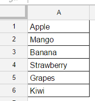
Here are the steps to create a drop-down list in Google Sheets:
- Go to the cell where you want the drop-down list.
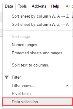
- Go to the Data tab and select the Validation option.

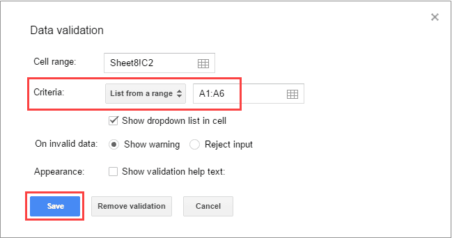
- In the Data Validation dialog box, make the following changes:
- Make sure Cell range refers to the cell where you want the drop-down list.
- In criteria, make sure ‘List from a range’ is selected and specify the cells that have the items (A1:A6 in this case).

- Click on Save.
This would instantly create a drop-down list in the selected cell. You will be able to see a small downward pointing arrow in the cell that indicates the presence of a drop-down list.
Now you can click on the arrow and the drop-down list would appear from which you can make a selection.

Note that this drop-down is dynamic. For example, if I go and change the source data (in cells A1:A6), the drop-down would automatically update.
Here is a video tutorial on creating a drop-down list in Google Sheets:
Also Read: Creating drop-down lists in Excel.
Get a list of Unique Items
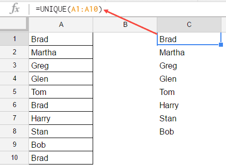
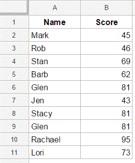
If you have a dataset that contains duplicates, you can quickly get all the unique items using the UNIQUE function.
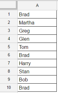
Suppose you have a dataset as shown below where there are duplicates:
To get all the unique names from this, select the cell where you want the names and use the following formula:
=UNIQUE(A1:A10)
This would instantly give you all the unique items (in this case names) from the list.
Note that this is an array function and you will not be able to delete one item from the unique. If you have to, you will have to delete the entire array.
Also Read: How to remove duplicates in Google Sheets.
Run Spell Check to Correct Misspelled Word
Nothing spoils the credibility of your work as fast as misspelled words.
Thankfully, Google Sheets have you covered here.
If you work with text data in Google Sheets, here is a quick tip to run spell-check in Google Sheets that will help you make your worksheet free of any misspelled words.
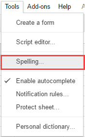
Here is how to run the spell-check in Google Sheets:
- Select the data on which you want to run the spell-check (or select the entire worksheet).
- Go to the Tools tab and click on the Spelling option.

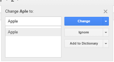
This will run the spell check on your data and show you any misspelled words it finds. You can then choose to correct it (manually or based on the suggestions) or ignore it.
Copy Sheets from One Google Sheets Document to Another
I am a fan of creating to-do lists and trackers. And Google Sheets is my weapon of choice.
Since I have created a lot of these lists and trackers, I decided to merge all my trackers into one single Google Sheets document and then use this master tracker instead.
And to do this, I had to copy sheets from multiple Google Sheets into one single Google Sheets document.
Below are the steps to create a copy of a sheet in another Google Sheets document:
- Open the Google Sheets document from which you want to copy the sheet. So these would be different trackers (lists) that I want to combine.

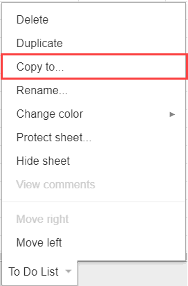
- Right-click on the sheet that you want to move to another master tracker Google Sheets document.

- Click on ‘Copy to..’ option.
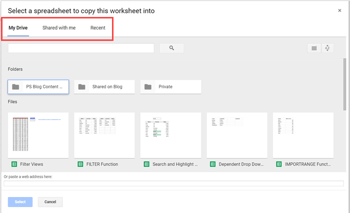
You will see a prompt that will tell you that the sheet has been copied. You can also open the target Google Sheets document, which now has the copied sheet.
Zoom In And Zoom Out in Google Sheets
This is one thing I miss in Google Sheets. It’s simple to zoom in and zoom out in Excel and is a useful feature to have.
Unfortunately, in Google Sheets, there is no way to Zoom just the Google Sheets work area. The only way to get this done is by zooming the entire browser window.
Here are the steps to Zoom In and Zoom in Google Sheets (if using Chrome browser):
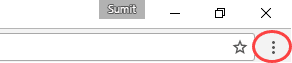
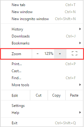
- Go to the top-right of Google Chrome browser and click on the ‘Chrome customize’ icon (shown below):

- Change the zoom level by using the +/- buttons.

You can read more about Zoom In and Zoom Out in Google Sheets here.
Insert Hyperlinks Using the HYPERLINK formula
HYPERINK function in Google Sheets allows you to quickly create a hyperlink using a URL. This can be useful when you have a list of URL and you want to quickly link these URLs to a given text.
Let me quickly cover the syntax of the HYPERLINK function:
HYPERLINK(URL, LINK_LABEL)
- URL – this is the URL that you want to insert as the hyperlink. You need to specify the full URL and need to enclose it within double-quotes.
- LINK_LABEL – this is the text that you would see in the cell. You need to specify the text in double-quotes.
Here is the formula that will insert the hyperlink of the Google homepage with ‘Google’ as the link label.
=HYPERLINK("https://www.google.com","Google")
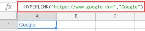
When you hover the mouse over the cell with the hyperlink, it would show you the link on which you can click. When you click on it, it will take you to that web page.
Transpose Data in Google Sheets
Just like Excel, Google Sheets also has the option to transpose data using the Paste Special options.
Suppose you have a dataset as shown below:
Transposing this data would mean that you would have the names in one row and the score below it in another row.
Here are the steps to transpose data in Google Sheets:
- Select the data that you want to transpose.
- Copy the data (right-click and select copy or use the keyboard shortcut Control + C)
- Select the cell where you want to get the transposed data.
- Right-click and within Paste Special, click on Paste Transpose.


That’s it!
This will transpose the dataset.
Note that when you use the above steps, it only transposes the data, but does not carry the formatting with it. You will have to copy the formatting separately.
Also, the transposed data is static. This means that in case the data changes, then you will have to repeat these above steps again to get the new transposed data.
You can read more about transposing data in Google Sheets here.
These 10 Google Sheets tips save me a lot of time daily and make me super-efficient.
I am sure you also have a couple of good Google Sheets tips up your sleeve. Would love to hear about it in the comments section.
Thank you for your tips.
How about drop-down for hours and minutes?
Excellent tips. Thanks.