The slicer is a really handy feature of Google Sheets. It enhances the power of Pivot Tables and Pivot Charts in Google Sheets.
With a Google Sheets Slicer, you can analyze your data much more interactively. You can create really amazing-looking and interactive reports and dashboards right within your Google Sheets worksheet!
In fact, once you’ve mastered the use of slicers, you’ll never want to go back to using regular filters!
In this tutorial, we will explain what Google Sheets slicers are. We will also demonstrate how to create and use Slicers in Google Sheets (with a practical example).
In order to understand this tutorial, you need to understand how Pivot tables and charts work. If you’re not familiar with these, it would be a good idea to first become familiar with the concepts and how they work. Since this is an integrated concept and can be quite difficult, we recommend taking a comprehensive Google Sheets course.
This Article Covers:
What is Slicer in Google Sheets?
A slicer is a Google Sheets tool that allows you to quickly and easily filter tables, pivot tables, and charts with just the click/ drag of a button. They float above your grid and are not tied to any cell, so you can easily move them around your window, align it, and position it however you like.
The slicer Google Sheets feature is called so, because it cuts through your data, similar to a filter, to give you customized data analytics. It is, however, better than a filter because it is much more visually appealing and user-friendly. Now let’s look at how to add slicer Google Sheets.
Download Our Example Spreadsheet
You can make a copy of our Example Spreadsheet to follow along with this guide. Now we’ll show you how to add and how to use slicer in Google Sheets.
How to Create a Slicer in Google Sheets (with Example)
To better understand how slicers work, let us try to take some sample data and create a slicer for it from scratch. Let us assume we have the following dataset, and we want Google Sheets to add a slicer:

This dataset has around 44 records of sales data for stores in three different regions – Central, East, and West.
From the above dataset, let us say we have two pivot tables – one that displays the sum of sales by each Sales rep and another that displays the number of units sold per product.

Let us say we also have a chart that displays a percentage of sales made by each Sales Rep, as shown below:

That means we have two pivot tables and a chart, all based on the same source data. Now we can create a slicer that can control all three entities at the same time.
Creating a Slicer Based on Region:
Let us create a slicer to filter all three entities (the two pivot tables and the chart) based on Region. For this, follow the steps below:
- Click any of the three entities (chart or pivot table) that you want to filter.
- From the Data menu, select the Add a slicer option.

- This will display the Slicer sidebar to the right of the Google Sheets window:

- You should also see a new slicer button created on top of the worksheet:
- Check if the data range (under the Data tab) displays the correct range for your source data. Remember this should contain the range for your original data (not the pivot table).

- Under the Column section, click on the dropdown menu to select the column by which you want the slicer to filter. Since we want to filter by Region, we will select the ‘Region’ option.


You should now see the name of the Region column as the title of the slicer:

We can use our Google Sheets pivot table slicer to filter out data in the pivot table based on the data for the region column in the original data.
How to Name the Slicer
When you create a slicer, it will usually come with the name of the column that is being used as the filter. For example, the slicer we created is for the Region column so it is called Region.
If you want to change the name of the slicer:
- Double-click on the slicer to open the slicer editing window.
- Go to Customize.

- Click the text box for the title and type in the new name for the slicer.

The name of the slicer will update immediately to the new title you added.
Customizing your Slicer
You can customize how your slicer looks from the Customize tab of the Slicer sidebar:

- Let us change the title of the slicer (the name that will be displayed on the slicer) to ‘Filter by Region’ to make it a little more descriptive for the user.

- You can also customize the font and background color of the slicer as you like. Let us change the background color of our slicer to orange.


Once you are done, your slicer is ready for you to interact with your pivot tables and charts.

How to Exclude Blank Data Rows from Slicer
If you have blanks in the data that you’re using for your slicer, you’ll usually get the option to filter out blanks in the slicer. If you click the slicer drop-down, you’ll see the Blank option with a tick on it.

Click on the Blank option to uncheck and click ok. This will filter out blanks in your data.
However, you can also choose to completely exclude blanks from your slicer. Here’s how:
- Click on your slicer dropdown
- Go to filter by condition.

- Click on the box and choose is not empty.

- Click OK.
The slicer will ignore cells that are blank when filtering out the data. In our example, we are filtering based on region therefore, if a row has an empty cell in the region, then data from that row will not be included in our pivot table.
How to Change Slicer Settings
If at any point you want to make changes to your slicer’s settings, you need to use the Slicer sidebar. Normally this is hidden from you. So if you want the Slicer sidebar to appear, follow the steps below:
- Click on the slicer that you want to edit.
- An ellipsis button (three vertical dots will appear on the right side of the slicer). Click on this icon/button.

- From the menu that appears, select ‘Edit slicer’.


This will make the Slicer sidebar appear once again, so you can make your required changes to the slicer.

How to Interact with a Slicer
To interact with your slicer, click on the drop-down arrow of the slicer to the right of the slicer title.
This should display a filtering menu quite similar to the menu you see on regular filters. You can use this to easily select which regions you want to include in your pivot table and chart summaries and which regions you want to exclude.

The results in the pivot tables and the chart will update when you change the filter applied in the slicer.
When the slicer filtering menu appears, you will notice you have the option to filter by values or by the condition.

Filter By Values
The Filter by values option lets you select the region values that will be included in the pivot table and chart results.
Let us say we want to see results for only the Central region stores. For this you will need to make sure to deselect all-region options and select only the Central region option, as shown below:

You will notice all the pivot tables and charts will now include results for only those stores that are in the Central region.

Similarly, if you include one more region, say the West region too, then your chart and pivot tables will now include results for only the West and Central regions:

This is how the worksheet would look now:

Filter By Condition
The Filter by condition option lets you add a condition that needs to be satisfied for a Region to be included in the results.
We will explain how you can use a slicer to filter by the condition in the following section, where we will create a second slicer to filter by Date.
Creating a Slicer based on Date in Google Sheets
It is important to understand that one slicer can filter by only one column. If you want to filter by more than one column, then you need to add multiple slicers, one for each column.
Let us say you want to further filter your summaries to display the sum of only sales made after 26/06/2019. For this, you will need to add one more slicer, this time based on the ‘Date’ column of the original dataset.
Follow the same steps to create this slicer as you had created the ‘Filter by Region’ slicer. You can give the new slicer the title, ‘Filter by Date’.

You can now filter your pivot tables and chart by condition with the following steps:
- Click on the drop-down arrow of the ‘Filter by Date’ slicer (to the right of the slicer title).

- This should display a filtering menu which you can use to enter the condition you want the dates included in your results to satisfy.

- Click on the ‘Filter by Condition’ option.
- This will display an input box that lets you select the kind of condition you want to enter.
- Click on the input box to display a dropdown list of options. Scroll down and select the ‘Date is after’ option.

- This will cause a new input box to appear just below. The new input box lets you select the date for your condition.

- Click on the new input box and select ‘exact date’.

- You should now see a third input box appear just below.
- Type in the date for your condition. Since we want to see the sum of sales made after 26/06/2019, type the date (in the appropriate date format):
- Scroll down the filter dropdown window and click OK.
- You will find that all the pivot tables and charts will now include results for only those stores that satisfy filters for both slicers.


So as you can see, you can filter your tables and charts using multiple slicers, and you can filter both by value and condition.
Depending on the filters applied, Google Sheets will hide or unhide entries/ results in all the tables and charts displayed in the current sheet that is based on the same base dataset.
Google Sheets Slicer vs Filter
Filters and slicers in Google Sheets perform the same function of filtering data, so it may be hard to differentiate between the two. However, there are some differences between a filter and a slicer:
- The difference between a filter and a slicer is usually physical, whereby a filter is usually locked to a row or column in the spreadsheet, while a slicer is a floating head that can reference any column to be used to filter data.
- Filters depend on the column that they are added to therefore, a filter can’t be changed, while a slicer can be changed to use any row or column of data in your data set for filtering.
This makes slicers sometimes more convenient to use than filters since they can be changed to use any column of data, and you can move the slicer around the spreadsheet for your own convenience.
Points to Remember
As a closing note, here are a few important points to keep in mind when using slicers in Google Sheets:
- You can connect a slicer to more than one table, pivot table, and/or chart.
- You can have only one slicer to filter by one column.
- You can apply multiple slicers to filter a single dataset by different columns.
- A slicer applies to all tables and charts on a worksheet, provided they have the same underlying source data.
- Slicers apply only to the active sheet
- Slicers do not apply to formulas on a sheet.
Frequently Asked Questions
What Does a Slicer Do in Google Sheets?
A slicer is a feature that lets you filter data based on a range of data or a condition in Google Sheets. The Google Sheet slicer option is particularly useful when working with pivot tables since you can filter data based on different columns from the original data. It also gives you a filter view so that you can tell what the data is being filtered against.
What is the Difference Between a Filter and Slicer?
Filters and slicers usually perform the same functions, so it’s hard to differentiate them. The difference is that a filter is usually locked to a row or column in the spreadsheet, while a slicer is a floating head that can reference any column for filtering.
What are the Limitations of a Silcer?
There are a number of limits when working with slicers in Google Sheets. They include the following:
- Slicers can’t be applied to formulas.
- When using multiple slicers from the same data source, they need to have the same number of cells in a column.
- You can only use one slicer per column. If you want to filter by more than one column, then you need to add multiple slicers, one for each column.
Final Thoughts
In this tutorial, I covered how to create, customize, and use a Google Sheets slicer.
I hope you found this tutorial useful! You can also have a look at our guide for calculated fields in Google Sheets.
Related:
- Using FILTER Function in Google Sheets (explained with Examples).
- Using Query Function in Google Sheets.
- How to Remove Duplicates in Google Sheets.
- How to Search in Google Sheets and Highlight the Matching Data.
- How to Highlight Duplicates in Google Sheets
- How to Insert a Pivot Table in Google Sheets