
If you’ve worked with Pivot tables, you would know that they are a great way to summarize large sets of data.
One, because they let you group data in a wide range of ways, and two, they let you use a number of summarizing metrics to analyze your data.
To add to their versatility, pivot tables also come with a ‘Calculated field’ feature, which lets you further customize your results with functions and formulas.
In this tutorial, we will demonstrate with an example of how you can use calculated fields in your pivot table to further harness its analytical power.
This Article Covers:
What are Calculated Fields in Google Sheets?
A pivot table provides a number of built-in metrics that you can use to analyze your data.
These include most of the standard summary metrics like average, median, variance, etc. However, oftentimes there are certain calculations that you need to get done, which might not be available in the built-in options.
This is where Calculated Fields come in. Calculated Fields let you process your data to provide more customized results in your Pivot table.
For example, what if you want to add a VAT to sales prices of items in a certain branch outlet? It would, of course, make sense to add a formula for this in your original dataset.
However, what if you want this to happen only in the pivot table, and leave the original data untouched?
Calculated fields can let you use custom formulas to display summary metrics within your Pivot table.
How to Use Calculated Fields in Pivot Tables in Google Sheets
Let us say you have the following dataset:

From the above dataset, let us assume you want to create a pivot table that will show the following:
- The total sales amount of different products.
- The amount obtained after adding 5% to the total sales amount for each product.
- The minimum number of units sold for each item.
In order to do this, you need to move step by step. That means you will need to:
- Create a Pivot table that will show the total sales amount for each product
- Add a Calculated Field that will display the customized formula results after adding 5% VAT to the total costs
- Add a Calculated Field that will display the customized formula after finding the minimum units sold for each product
Let us go over these steps one by one.
Creating a Pivot Table to Show Total Sales Amount for Each Product
To create the pivot table that will show the total sales amount by product, here are the steps that you need to follow:
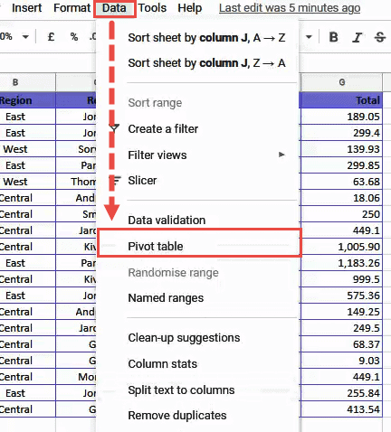
- Click on the Data menu from the menu ribbon.
- Select the Pivot Table option from the drop-down menu that appears.

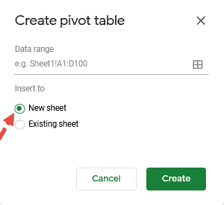
- You should now see a box asking if you want to insert your pivot table on the existing sheet or on a new sheet. Select the option that you prefer. For clarity, it is always better to create one in a new sheet.

- Click on the Create button.
- This should create your pivot table, either on the same sheet or a new sheet, depending on what you had opted for in step 3.
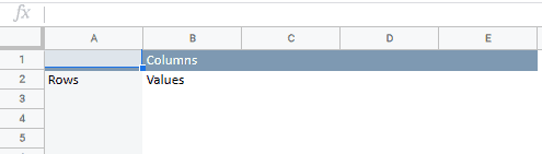
- Your pivot table at this point should look like the screenshot shown below:

- There should be a grid displaying ‘Rows’, ‘Columns’, and ‘Values’.
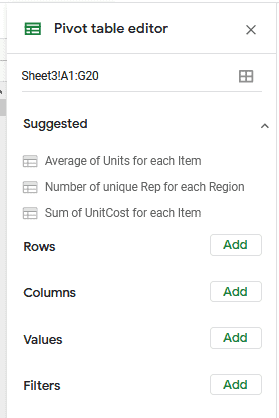
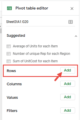
- You can now start filling your pivot table with your required data. On the right side of the window, you should see a Pivot Table Editor. This will help you specify what should go into your pivot table.

- We now want our pivot table to have two columns (initially) – The Item and the total sales price. So from the ‘Rows’ category, click ‘Add’.
- From the dropdown list that appears, select Item. This will add each unique item name to individual rows of your pivot table.

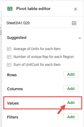
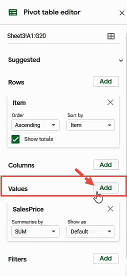
- Next, we want to see the total sales amount for each item. So from the ‘Values’ category, click ‘Add’.
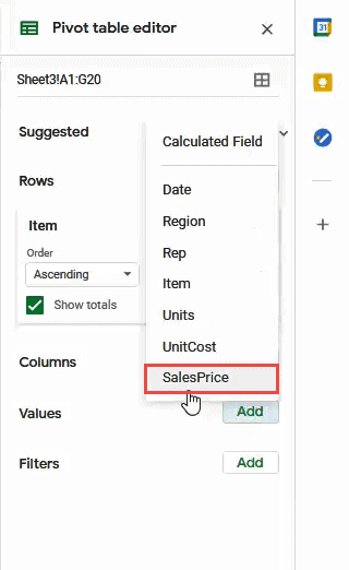
- From the dropdown list that appears, select ‘SalesPrice’. This will display the sum of all sales prices for each item.


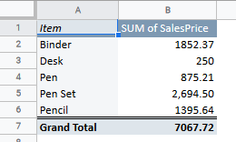
This displays the total sales amount per product, as shown below:
Now, what if you also want to see what happens when you add a 5% VAT amount to the total sales amounts of each product?
In the Values category, if you click on the dropdown list under ‘Summarize by’, you will notice that there is no option for adding 5%.
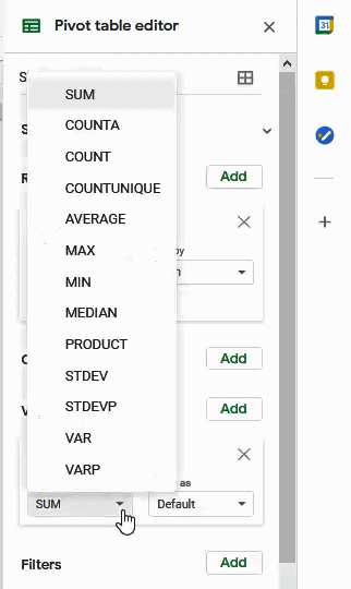
That means you will need to define the custom calculation yourself. This can be easily done by adding a calculated field.
Adding a Calculated Field Summarized by SUM
Now you want to add 5% to the total sales amount of each item and display it in a new column. Since the calculation is to be performed on the total sales amount (the SUM of the SellingPrice values for each item), your calculated field will need to be summarized by SUM.
Here are the steps you need to follow if you want to add a 5% VAT to the total sales amount for each product:
- Click on any cell of your pivot table.
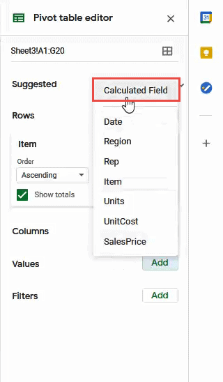
- From the ‘Values’ category, click ‘Add’.
- From the dropdown list that appears, select the Calculated field option.

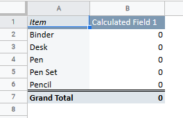
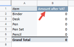
- You will now see a new column in your pivot table that says ‘Calculated Field’.

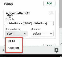
- You can go ahead and change this name right from the Pivot table. Let us rename it to ‘Amount after VAT’.

- You should also see some options for your calculated field in the Pivot table editor.
- In the input box under Formula, you can enter the formula that you want for your calculated field results.
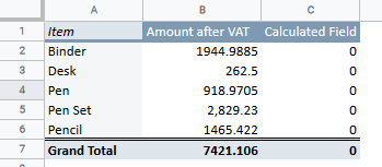
- Since you want to display the amount obtained after adding 5% to the total sales amount, type the formula: =SalesPrice + ((5/100) * SalesPrice). Notice the variable ‘SalesPrice’ here refers to the ‘SalesPrice’ column in the original dataset.
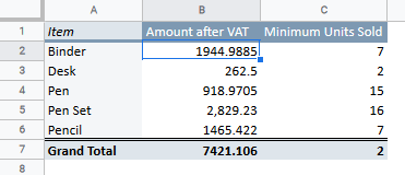
- This should now display the results of our custom formula in the new calculated field created.
Note: Since we wanted to add the VAT amount to the total sales for each product, we left the ‘Summarize by’ field set to the default value, ‘SUM’. If you click on the dropdown list under ‘Summarize by’, you will notice that the only two options you get are ‘SUM’ and ‘Custom’.
If you want to display the minimum units sold for each item then you would need to use individual ‘Units’ values from the original dataset in your custom formula, instead of the SUM. We will see how to do that in the following section.
Adding a Calculated Field Summarized by ‘Custom’
We now want to find the minimum number of units sold for each product. Note that we want to use the individual units sold on a particular day for each product, not the SUM of the units sold. This means our calculated field cannot be summarized by SUM. There is another option for ‘Summarize by’ and that is the ‘Custom’ option.
Here are the steps you need to follow if you want to find the minimum units sold for each product:
- Click on any cell of your pivot table.
- From the ‘Values’ category, click ‘Add’.
- From the dropdown list that appears, select the Calculated field option.

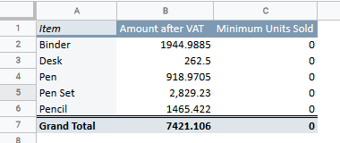
- You will now see a new column in your Pivot table that says ‘Calculated Field 2’. You can go ahead and change this name right from the Pivot table. Let us rename it to ‘Minimum units sold’.

- You should also see some options for your calculated field in the Pivot table editor.
- In the input box under Formula, you can enter the formula that you want for your calculated field results.
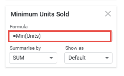
- Since you want to display the minimum units sold, type the formula: =MIN(Units). Notice the variable ‘Units’ here refers to the ‘Units’ column in the original dataset.

- Click on the dropdown list under ‘Summarize by’ and select ‘Custom’.

- This should now display the results of our custom formula in the new calculated field created.

Note: Since we wanted to find the minimum units sold for each product, we changed the ‘Summarize by’ field to ‘Custom’, instead of SUM.
Important Points about Calculated Fields
Calculated fields provide a lot more flexibility and versatility to pivot tables. However, it still has certain limitations. Therefore, it is important to keep in mind certain points when creating calculated fields.
- Your calculated field formulas refer to only cells of your original dataset. They cannot refer to the pivot table’s totals or subtotals.
- You need to use the field names of your dataset in the calculated field formulas. You cannot refer to individual cells with their address or cell names.
- It is important to ensure you provide the correct variable name for the fields in your formula. If your field name has more than one word with spaces in between, then you need to enclose the variable name in single quotes when including it in the calculated field’s formula.
In this tutorial, we showed you, some simple examples of how to use pivot tables with calculated fields.
As you can see, calculated fields help make your pivot tables more powerful, as they let you customize your summaries and results to your liking. We hope you enjoyed this tutorial and found it helpful.
Other Google Sheets you may also like: