How to Create and Use Filter Views in Google Sheets

Watch Video – Creating and Using Filter Views in Google Sheets

Google Sheets has this amazing functionality to collaborate with other users.

However, one issue when multiple people are working with the same file is that when someone changes the data, it gets changed for everyone who is working on that data.

Filter Views in Google Sheets can help you tackle this problem.

What are Filter Views in Google Sheets?

A Filter View is a view (or arrangement of data) that you can save for future viewing/use.

For example, suppose you have a dataset as shown below:

This is the store wise sales data has four regions – East, West, North, and South.

Now if you’re working with collaborators who also have access to this data, any changes you do in this would also impact what they see.

So instead of changing the original data, you can create a Filter View.

A filtered view sits above the original data.

You can filter or sort the data according to your need and then create a ‘filter view’ of that data. This will ensure that the original data remains as is, and you still have access to the ‘filter view’ data in case you need it in future.

And the best part of ‘Filter Views’ is that you can also share it with other collaborators (we will see how to do this later in this tutorial).

How to Create a Filter View in Google Sheets?

Suppose that I have the same sales data shown above, and I want to analyze the data to get the data for the following:

• Stores in East region that have sales of Product A less than 500
• Stores in West region that have sales of Product A less than 500
• Stores in North region that have sales of Product A less than 500
• Stores in South region that have sales of Product A less than 500

This would need creating four different ‘Filter Views’ – one for each region.

Here are the steps to create Filter Views in Google Sheets:

1. Select the dataset.
2. Go to the Data tab.
3. In the Filter views option, click on ‘Create new filter view’. You would notice that the row/column header turn dark-gray.
4. In the bar above the row header, enter a descriptive name for the filter. In this case, I will name is ‘East with Sales Less than 500’.
5. Make sure the Range refers to the right range. It automatically picks the selection range, but you can change it if you want here.
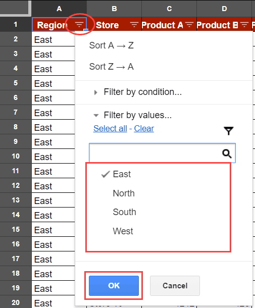
6. Click on the Filter icon for Region column, and filter all the East records.
7. Click on the Filter icon for Product A icon, click on ‘Filter by condition’, and filter all record with a value less than 500.

The above steps would create a Filter View in Google Sheets that you can use to see the stores in East that are selling less than 500 of Product A.

You can close the Filter View by clicking on the close icon at the right of the gray bar.

To create other Filter Views, follow the above steps again.

Accessing Different Filter Views in a Google Sheets Document

To access the existing filter views in a Google Sheets file, follow the below steps:

• Go to the Data tab.
• Hover your cursor over the ‘Filter Views’ option in the list.
• Click on the Filter View you want to access.

This would instantly change the color theme of the row/column headers and open the selected filter view.

Sharing Filter Views with Others

The best part about Filter Views is that you can share it with other collaborators.

To share a ‘filter view’, you first need to open it, and then copy the URL of the file and share it with the other collaborators.

You will notice that when in filter view, the URL of the Google Sheet gets an additional &fvid=########

This Filter View id is unique for each view and allows you to share a unique URL with a collaborator.

In case the collaborator has the permission to edit, he/she can make view as well as make edits to the Filter Views. Once the edits are made, it would be saved and applied for all the collaborators.

In case the person you shared this with has only viewing rights, they will only be able to view the filters. If they try and filter the data or sort it, it will be temporary and only visible to them. This will not change the original Filter View. When someone with only viewing rights filters/sorts data, the name of the Filter View changes to something like ‘Temporary Filter 1’.

Deleting Filter Views

If you create a ‘filter view’ that you no longer need, you can easily delete it using the below steps:

• Go to the Data tab
• Hover your cursor over the ‘Filter Views’ option in the list.
• Click on the Filter View you want to delete.
• Click on the Gear icon.
• Click on Delete.

The above steps would delete the active Filter View.

In the gear icon drop down, you also get the following options:

• Rename: Use this to rename the current Filter View.
• Update Range: Use this to update the range for which the Filter View is created. This will help when someone adds/deletes data in the original data set and you want to update the filter view accordingly.
• Duplicate: Use this to quickly duplicate filter views. This is useful when you want to create multiple ‘Filter Views’ with similar data filtering/sorting.

Creating Clickable Links to Open Filter Views in Google Sheets

Now if there are multiple filter views that you have created in Google Sheets, it can be helpful to create clickable links in cells to access these views quickly.

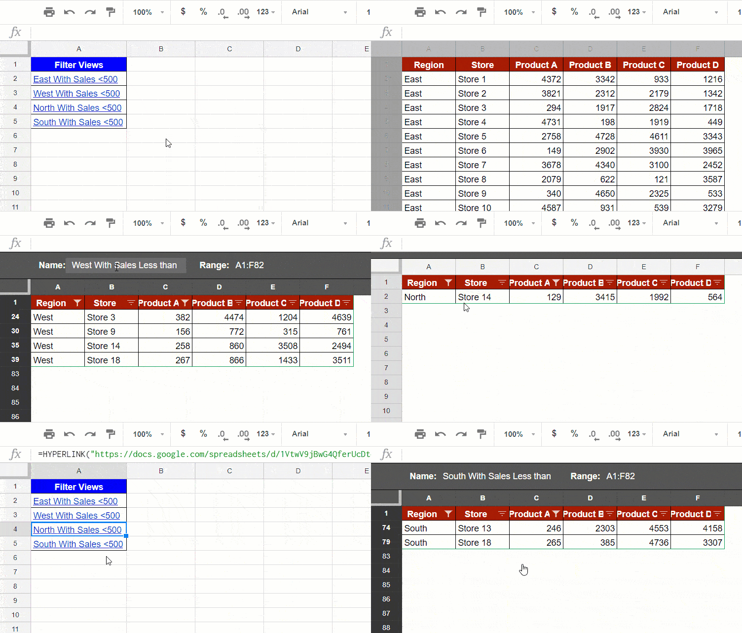
For example, if I am a manager and I want to quickly see which stores underperformed in the four regions, I can just click on a link, and it instantly opens that specific filter view. Something as shown below:

Here is how to create this links:

• Go to the Data tab.
• Hover your cursor over the ‘Filter Views’ option in the list.
• Click on the Filter View for which you want to create a link.
• Copy the URL of the Google Sheet document, while the Filter View is active.
• Close the Filter view.
• In a cell, use the formula: =HYPERLINK(“URL”,”Text”), where URL would be the one you copied in step 4, and Text would be the content of the cell that you want visible to a user.

The above steps would create a hyperlink in the cell that will open the specified Filter View when clicked.

You can use this as a part of the dashboard or summary sheet, where if one wants to check out the filter views data, they can simply click on the link (as shown below).

You May Also like the Following Google Sheets Tutorials:

• Using FILTER Function in Google Sheets (explained with Examples).
• Using Query Function in Google Sheets.
• How to Remove Duplicates in Google Sheets.
• How to Search in Google Sheets and Highlight the Matching Data.
• How to Highlight Duplicates in Google Sheets
• How to Insert a Pivot Table in Google Sheets
• How to Use Slicer in Pivot Tables in Google Sheets