An Easy Pivot Table Google Sheets Guide (Learn in 5 Mins)

Spreadsheets provide a great way to work with data. They help you keep your data organized to get good insights from it. Google Sheets gives the added facility of Pivot tables that makes the data analysis process even more powerful.

This pivot table Google Sheets tutorial will give you the jumpstart you need to delve deeper into your data and do some serious data processing magic. It will also show you some of the ways on how to use pivot tables in Google Sheets. Read on to learn how to do a pivot table in Google Sheets.

What are Pivot Tables?

A pivot table takes a large data set and helps summarize and draw conclusions from it.

A small spreadsheet with little data makes it easy to read, understand, and make inferences from. But as the data gets bigger, all you see are a lot of numbers. It then becomes difficult to draw conclusions from your data.

How do Pivot Tables Work?

Let us see a use case. Consider the sample data in the image below. It consists of details about employees’ sales in an imaginary stationery chain. At first sight, all we see are lots of numbers, dates, and text. It’s quite difficult to make any sense of this data.

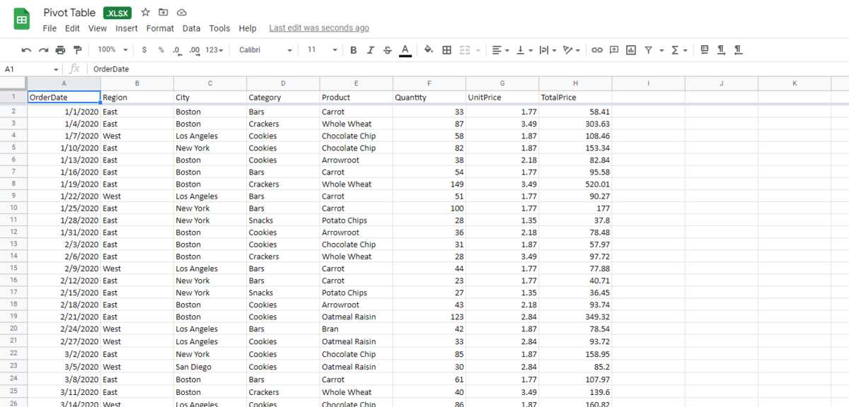
But by using pivot tables, you can narrow down an extensive data set like this and visualize relationships between the data points quite easily. For example, you could use a pivot table to answer questions like:

• Which salesperson brought the most revenue for a specific month?
• Which region made the most sales?
• How many units of Pencils were sold?
• Which sales reps failed to reach their targets?

Now, of course, it is possible to analyze the data using formulas and functions, but Pivot tables can get your work done much quicker and easier, and with minimum human error.

Pivot Table Google Sheets: The Benefits

Here are some of the reasons more, and more people love the power of Pivot Tables:

• As mentioned above, the Pivot table can help analyze data more efficiently
• They are quicker to put together and easier to explore than formulas and functions.
• They are flexible and versatile. Using Pivot tables, you can narrow down your data to just the important data points and add more to it as and when required.
• They even allow you to summarize data using aggregates, formulas, and functions if needed.

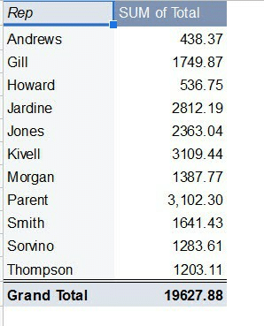
In the above use case, we can easily use Pivot tables to narrow down the data to show us just how much each sales rep sold in total.

There is a lot of functionality to pivot tables that you can use to analyze data.

You can use these pivot tables to create a Google Sheets pivot chart. You can also insert slicers in your pivot table. A slicer puts filter control on the face of the sheet that users can use to apply filters. You can get specific data from the pivot table or group data by months and other categories.

You can also add calculated fields in your pivot table in Google Sheets using the pivot table editor. These let you perform other calculations that are not among the defaults in the pivot table editor.

How to Insert Pivot Tables in Google Sheets

Here’s how to insert a pivot table in Google Sheets and use it to analyze data in our use case. We obtained this sample data from the following page:

https://www.contextures.com/xlSampleData01.html

The data is free to use and download, so you can download it too, and convert it to Google Sheets in order to follow our tutorial.

Step 1: Select all the cells in the given spreadsheet. You can do this quickly by selecting the first cell on the top-right, then pressing the shift key while simultaneously clicking the last cell at the bottom right. Make sure you also select the column headers.

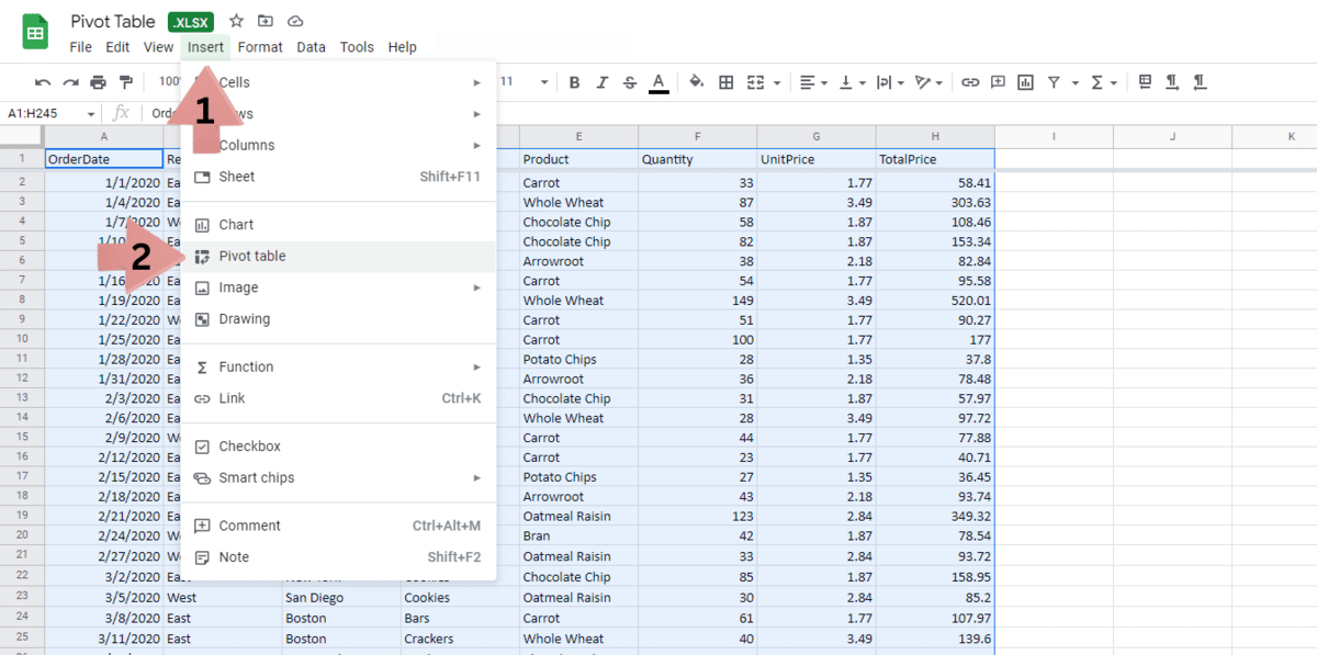
Step 2: From the Insert menu, select Pivot Table.

Step 3: You will be asked if you want to insert your Pivot Table in a new sheet or into your existing sheet. It’s usually better to use a fresh sheet. So select the “New Sheet” option.

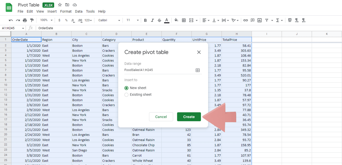
Step 4: Click on the Create button.

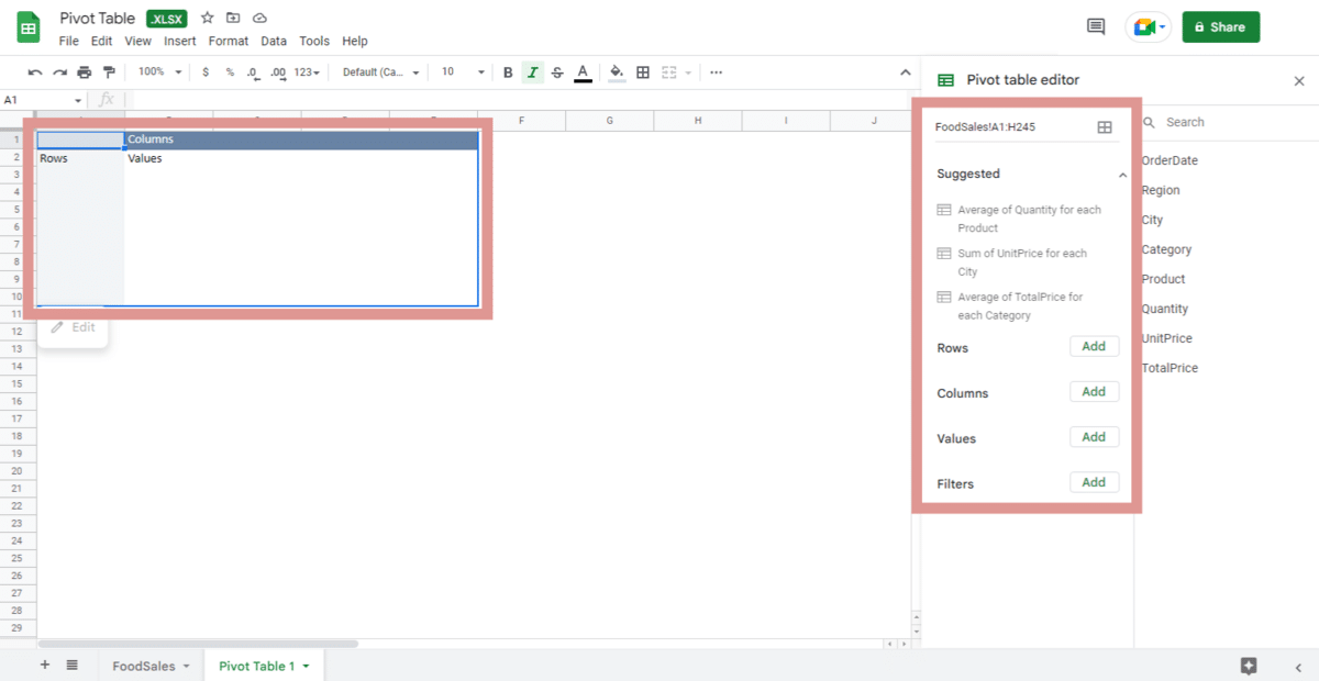
You will see your Pivot table created in a new Spreadsheet named Pivot Table 1. You can go ahead and rename it to something else if you need to.

Step 5: On the right, you will see a sidebar, which is the “Pivot Table Editor”.  Here you will find some Pivot tables that Google Sheets automatically suggests based on your selected data. You can choose to either accept the suggestions (if you feel they answer your needed questions aptly), or you can create your own Pivot tables with the data that you require.

How to Use Pivot Tables Suggested by Google Sheets

Google Sheets has the ability to build pivot tables automatically through suggestions. If you click on any of the suggestions provided, Google Sheets will automatically create your initial pivot table. Let’s take a few minutes to first explore some of these suggestions.

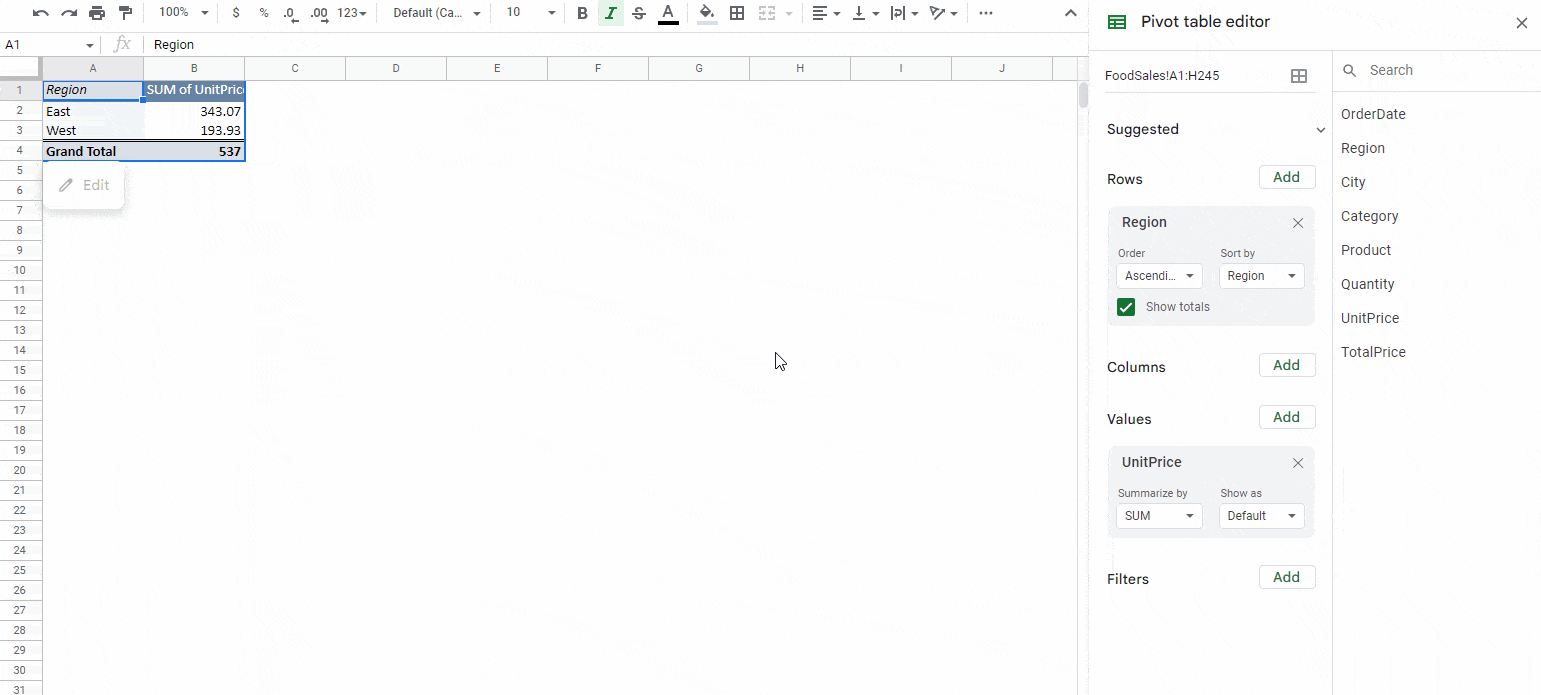
One of the suggestions is a Pivot table that shows the average units sold by each sales rep. If you click on this option, you will get a Pivot table that can help you easily find out which sales rep sold the most units on average, how each of them stacks against each other and who possibly deserves a promotion this year!

Another suggestion is the sum of the unit cost for each region. This will give you a table with each region and the corresponding total of unit costs. Through this, you can get a sort of idea about how each region has been doing (sales-wise).

Note that you can use the suggested Pivot table and add your own rows and columns to customize it.

For example, it makes more sense to see the number of units sold region-wise rather than the total of unit costs. So, you can delete the “Unit Cost” column by selecting the cross corresponding to the “Unit Cost” option under “Values”.

This will delete the SUM of Unit Costs column from the Pivot Table.

You can then click on the Add button next to “Values” and select “Units” from the dropdown.

How to Create a Pivot Table Manually in Google Sheets

If the suggestions given by Google Sheets do not match your requirements, you can also manually build your own Google Sheet pivot table.

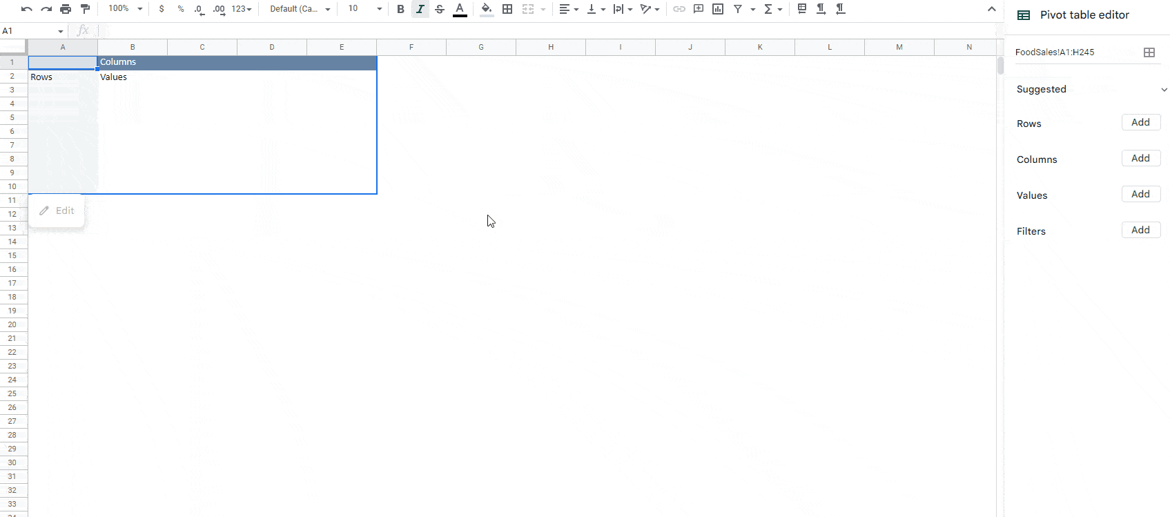
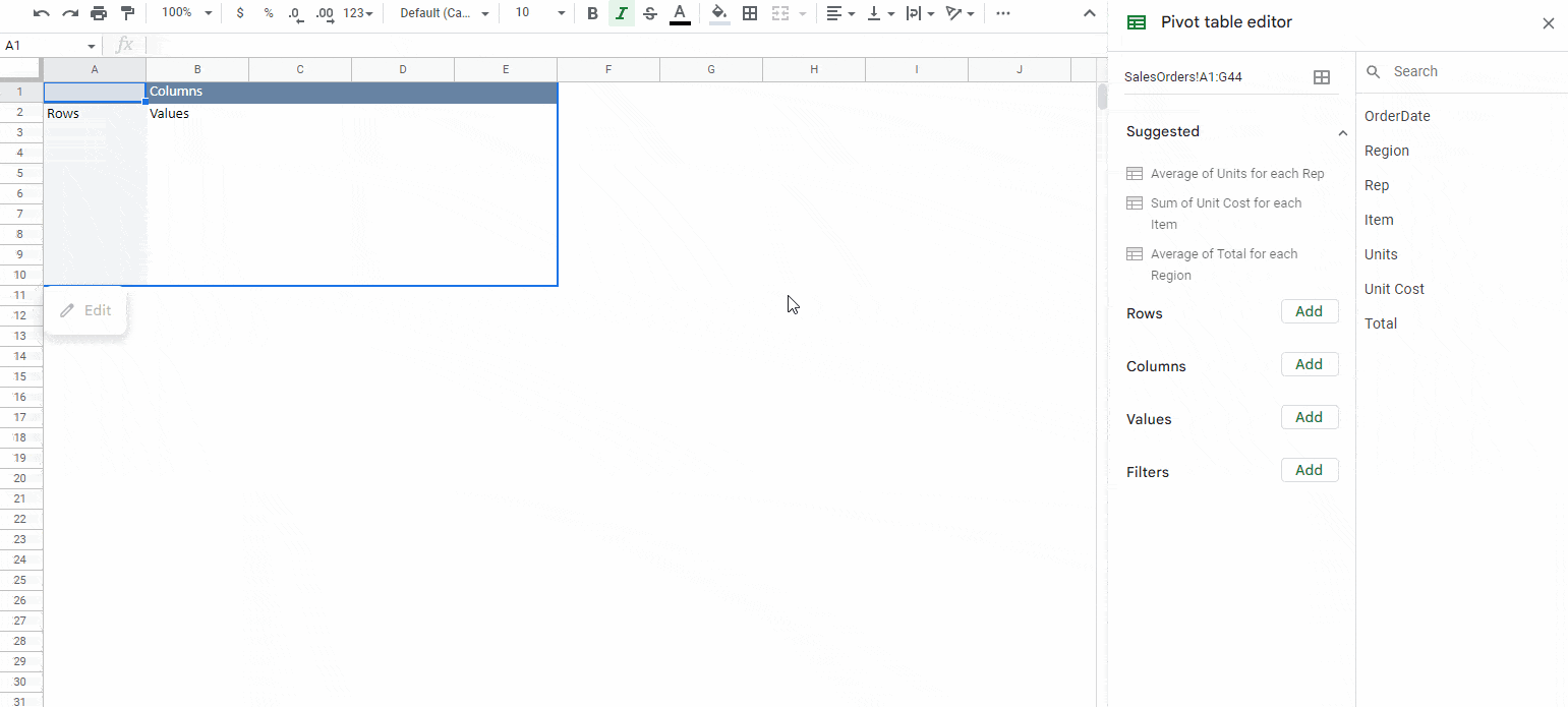
The Pivot Table Editor (on the right sidebar) also gives you options to insert data to your Pivot table according to your requirements.

You will see 4 insert options here:

• Rows
• Columns
• Values
• Filters

Let’s try to make a custom Pivot table to perform analysis like this:

How many sales did each sales rep make for different types of items sold in the year 2018?

To answer the above question, here’s what we need in each of the dimensions:

• We want the Pivot table to display the names of the sales reps in each row.
• We want to display the different items sold across each column.
• We want the value of the total sales in cells where each Sales Rep name meets the item name.
• We want filters to display only the values for the year 2018. Filters let you see parts of the data while keeping unnecessary parts of it obscured.

Now let’s start building our Pivot Table.

Inserting Rows:

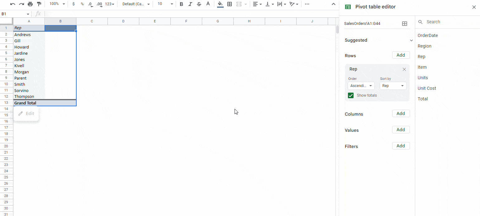
To display the names of sales reps in each row, click on the Add button next to “Rows” and select “Rep” from the dropdown. The Pivot table will pull the names of all the Sales reps from your original data.

Notice that the Pivot table takes the names of the sales reps, removes duplicates and displays them in alphabetical order in Column A.

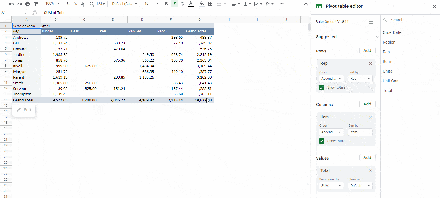
Inserting Columns:

Next, we want to display different items sold across each column. For this, click on the Add button next to “Columns” and select “Item” from the dropdown. The Pivot table will display the names of different items along each column, without any repetitions.

So now your table is starting to take shape. You have the sales reps along the rows and item types along the columns.

Inserting Values

To populate the individual cells of the Pivot tables, we need the values of total sales made by each sales rep for each item.

Click on the Add button next to “Values” and select “Total” from the dropdown.

You will now see the total sales made for each type of item for a given sales rep.

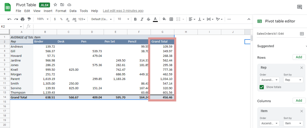
If instead of total sales you want to see the average sales, click on the dropdown below “Summarize By” under “Total” and select “Average” from the dropdown.

The totals in each cell should now be replaced by the average sales made for each type of item for a given sales rep.

You will also find the “Grand Total”, calculated automatically for each item at the bottom of the Pivot table. The Grand Total for each sales rep is displayed on the rightmost column of the table.

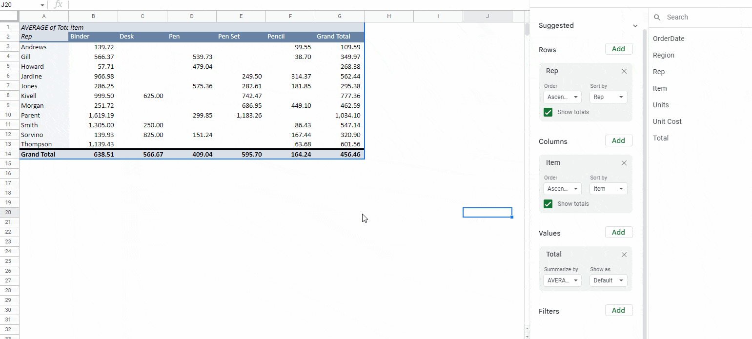
Adding Filters

Our Pivot table has already started giving a lot of useful insights. The only thing left to do is ensure that we get the average sales for just the year 2018. For this we use filters.

1. To add a filter, click on the Add button next to “Filters” and select “OrderDate” from the dropdown.
2. Under OrderDate, click on the dropdown below “Status” .
3. Click on “Filter by Condition”
4. In our original table, there are only dates for the year 2021 and 2022. Since we want values for just 2021,
   • Select “Date is before”.
   • Under this, you will see another dropdown next to the word “today”. Click on this and select “exact date”.
   • Type the date 01/01/2022 in the input box.

This will ensure that the averages only consider all the dates before 1st Jan 2022 (Which is just all the dates of the year 2021!)

1. Click OK to update the Pivot table.

That’s it!

We now have a Pivot table that answers our question: How much sales did each sales rep make for different types of items sold in the year 2021?

Refreshing Values

Usually, the pivot table should automatically update, but there are some times when you may need to refresh it. Check out our other guide here on how to refresh pivot tables in Google Sheets.

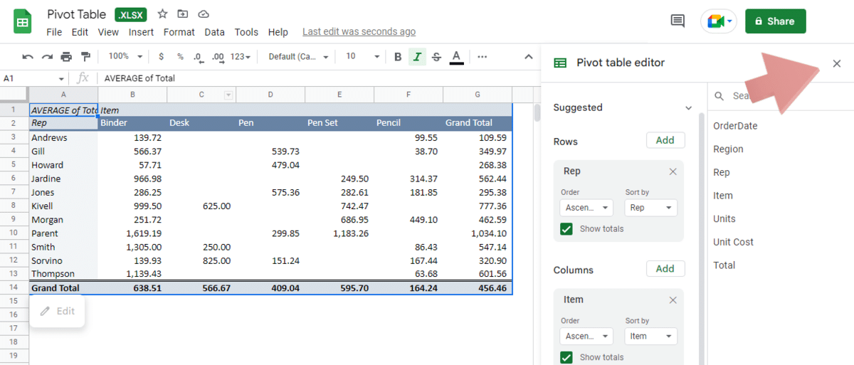
How to Hide the Pivot Table Editor in Google Sheets.

It is possible to close your pivot editor tab once you are done using it by clicking on the x at the top of the table editor.

In case you wish to access the pivot table editor again you will find an edit button at the bottom of your pivot table. Clicking it will reopen the pivot table editor.

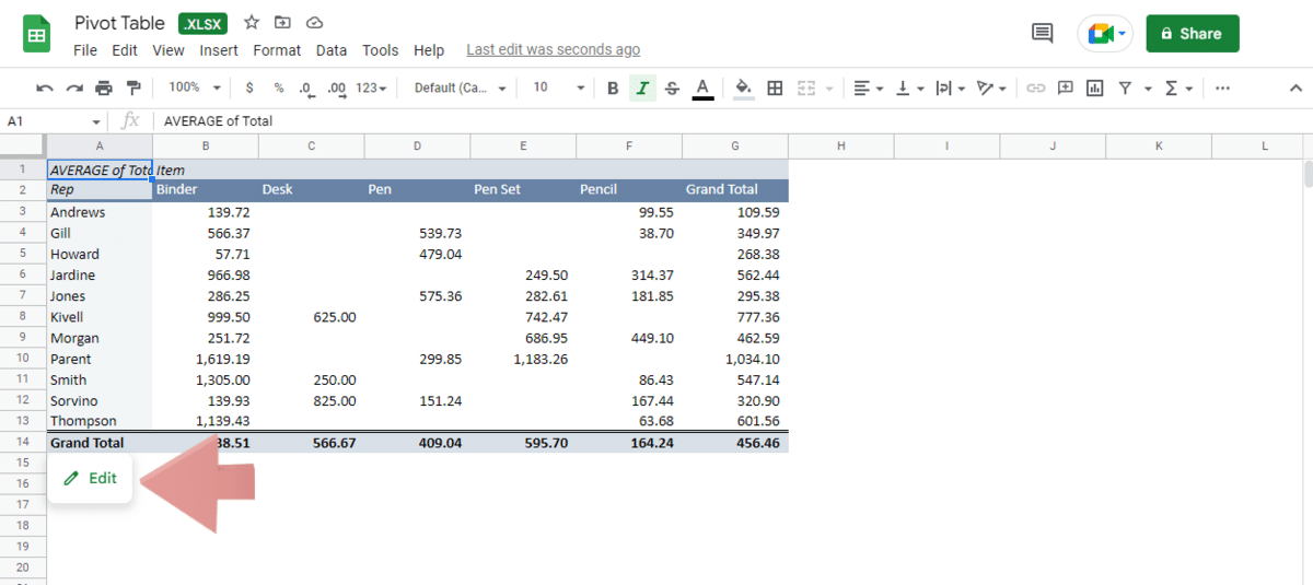
However, you can’t hide the pivot table editor from other users since they will still be able to access it with the edit button.

Pivot Tables in Excel vs in Google Sheets

There are a couple of differences between the spreadsheet pivot table in excel and in Google Sheets:

• Google Sheets gives you suggestions for your pivot table unlike excel
• Excel has more options for customizing your data while Google Sheets has less options which are easier to use.
• You can import pivot table to Google Sheets from excel by selecting import from the Google menu and selecting the file. To import to excel all you need to do is to download the file from Google Sheets as an Excel file.
• Excel does not automatically update the existing pivot table when you change the source data so you will have to refresh the pivot table manually whereas Google Sheets automatically updates the pivot table when you change the source data.
• Some functions also work differently in Excel’s pivot table compared to Google Sheets pivot chart. For example if you want to get data from the pivot table in sheets you can just type the equal sign and the cell reference and it will obtain the data, In excel you have to use the get pivot data which is a bit more complicated than the Google Sheets way. However, if you were to change or update your pivot table in Google Sheets then that will affect the cell references and return the wrong data while in excel the get pivot table function will update with the changes in the existing pivot table and give you the correct values.

Read more: Google Sheets vs Excel

Frequently Asked Questions

Do Pivot Tables Update Automatically in Google Sheets?

Yes, pivot tables do update automatically whenever you add or change the source data in Google Sheets. It also updates formulas automatically if you add or remove the rows and columns used in the pivot table data.

What is the Difference Between a Table and a Pivot Table?

A pivot table is able to summarize data while a table only represents the raw data that has been input to it. You have to insert pivot tables Google Sheets while for a normal table you just have to input the data.

How Do You Aggregate Types in a Google Sheets Pivot Table?

Aggregation types are used in Google Sheets to summarize data by calculating the sums, averages, mediums and more. The pivot table usually does some of these automatically like the average and the sum by creating a suggested table with aggregated data.

You can also create a new aggregation table in the summarize drop down menu which gives you a number of functions including sum, max, min and median.

How Do I Create a Pivot Table in Google Sheets?

Here’s how to make pivot table on Google Sheets:

1. Select the data for your pivot table
2. Navigate to Insert > Pivot table
3. Click New sheet
4. Click Create
5. Make choices inside the Pivot table editor

Why Would I Use a Pivot Table?

Pivot tables make it much easier to interpret large data sets, which also reduces the risk of human error when transferring data.

Can You Do a Pivot Table in Google Sheets Mobile?

No, unfortunately, you can’t build one. However, you can view the ones you make on the desktop version of Google Sheets.

How Do I Create a Pivot Table in Google Sheets With Multiple Sheets?

You can’t. You have to get all your data into one sheet first. You can simply copy and paste into a new sheet, or use the QUERY function to import the data from the two other sheets.

Conclusion

Pivot tables make things so much easier when we want to sift through large amounts of data or want to see the bigger picture. With all of the information we want right in front of us, we can now answer almost any questions we have about our original data.

In this article we have shown you the way for creating a pivot table in Google Sheets and how to use a pivot table. We hope this pivot table Google Sheets guide taught you everything you need to get started.

So, go ahead, give it a try, unlock the power of Google Sheet Pivot Tables, and make unlimited discoveries about your data. You should be able to make a wide range of pivot tables now, from simple to advanced pivot tables, in Google Sheets.