Whether you’re a beginner or an expert spreadsheet user, you’ve come across a formula parse error at some point. While these issues are frustrating, I’m here to walk you through solving and preventing common formula parse errors like #REF, #DIV, #ERROR, and #NUM.
Let’s get started!
This Article Covers:
What Is a Formula Parse Error?
A formula parse error occurs when Google Sheets can’t understand your formula. There are plenty of reasons this might occur, including:
- Your formula has typos
- There are more/fewer parameters than required for a specific function
- At least one entered parameter is different than what’s required
- Your formula’s cell references might be out of bounds.
- You’re trying to perform a calculation that is mathematically impossible.
Regardless of the reason, Google Sheets struggles to fulfill your formula’s request. As such, it returns an error message.
Thankfully, Google Sheets provides suggestions as to what might be wrong with the formula. In turn, this can help you break it down and detect the root of the problem.
The Most Common Formula Parse Errors
The most common error messages you’re likely to see include:
1. #N/A Error
This usually occurs when a particular value the formula needs isn’t present. In other words, the value is “not available” for the formula to work on.
For example, if you’re looking for a value – and that value does not exist in the given range – you will most likely see a #N/A error.
In the image, the VLOOKUP function needs to find the value ‘Tom’ from the range A:B. Since the value ‘Tom’ doesn’t exist in the range, the function returns a #N/A function. This indicates that the value ‘has not been found.’
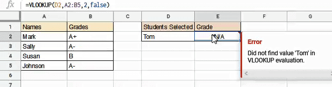
Note: This problem is often encountered when using lookup formulas like VLOOKUP in Google Sheets.
How to Fix an #N/A Error
The #N/A error doesn’t always signify a problem with your formula. However, a certain circumstance (i.e., the absence of a value) will result in an error.
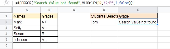
To fix it, combine the formula with an IF statement that displays a custom message. I recommend using the IFERROR function to handle this issue. For example, I rectified the issue by using an IFERROR statement to display a “Search Value not found” message instead of an #N/A error:
2. #DIV/0 Error
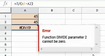
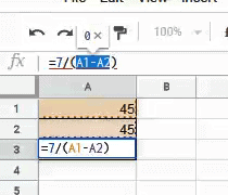
The #DIV/0 error occurs when a number in the formula is divided by zero. This makes no mathematical sense. For example, say that you’re trying to divide a value by a function or operation that results in a 0 value: You will get a #DIV/0 error.
In the image below, I’m trying to divide the number 7 by the difference between values in A1 and A2. This results in 0. Since it isn’t possible to divide 7 by 0, the formula returns a #DIV/0 error.
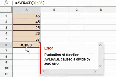
This error also happens when you try to apply the AVERAGE function to a range of blank cells. It occurs because the AVERAGE function needs to divide the SUM of the values by the number of the values. If the range is blank, it’s equivalent to dividing by 0.
How to Fix the #DIV/0 Error
To resolve this error, you can try to understand why your denominator is a ‘0’ value. Investigate parts of the denominator in the formula bar. The result of the calculation is a little pop-up (right on top of the formula bar). Once you determine the cause, make changes to your formula accordingly.
If that doesn’t work, check whether any part of the formula’s denominator links to a blank cell or range. If so, you can fill the required values in the cell or select the required range for the formula.
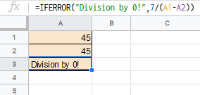
To avoid problems like this altogether, use the IFERROR statement to display a particular message whenever you encounter an error:
3. #REF! Google Sheets Error
This error occurs when you have an invalid reference in your formula. There may be different types of invalid references:
Missing Reference
This kind of #REF! error occurs when you’re referencing a missing cell in your formula. In the image below, we have two values in cells A1 (45) and A2 (50). I’ve used the formula =A1+A2 to find the sum of the two numbers in cell A3.
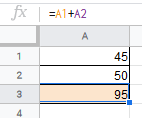
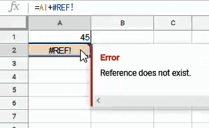
But what happens if we delete row 2? The value in cell A2 would go missing, causing the formula in cell A3 to return a #REF! Error.
Circular Dependency
This kind of #REF! error occurs when your formula may reference itself. In the image below, we used the formula =SUM(A1:A3) in cell A3. This means the formula – in addition to referring to values in A1 and A2 – also refers to itself.
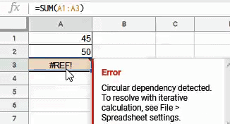
Therefore, the function goes around in circles as an input and output cell, resulting in an infinite loop (and a system crash). The formula then detects the circular reference and returns a #REF! error.
Lookup That’s Out of Bounds
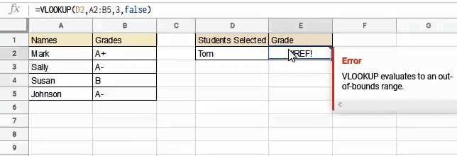
This kind of #REF! error occurs when you use the LOOKUP function to reference a cell that’s outside the bounds of the VLOOKUP range parameter.
The VLOOKUP formula attempts to find the search parameter in the third column of the source table (even though the specified range parameter only consists of 2 columns).
Since you’re trying to return a value outside the range specified by the formula, it returns a #REF! error.
How to Fix the REF Error
To find out what kind of #REF! error your formula has, you’ll need to read the error message. If there are missing references, you can see the erroneous reference in the formula bar. The reference causing the problem will be replaced with #REF!
Once you’ve identified which cell is missing, you can replace the #REF! with the correct cell reference.

If there’s a circular dependency issue, you’ll first need to identify the range of cells in the formula. Next, you’ll need to change it to ensure it doesn’t include the current cell, too.
Finally, if there’s an out-of-bounds error, either make sure the search term exists in the search table or make the required changes to the search term itself. You can also avoid this type of error from happening by using the IFERROR function.
4. #VALUE! Google Sheets Error
This error occurs when one or more parameters in your formula are a different type than what’s expected. If a function only accepts numbers as a parameter – but you have a text value in the cell being referenced – you’ll end up with a #VALUE! Error.
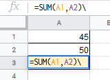
In the image below, a backslash character (\) was mistakenly added to the end of the number in cell A2. When we use the formula =A1+A2 in cell A3, we’ve added a number to a text value, making it invalid. Therefore, the formula returns a #VALUE! Error.

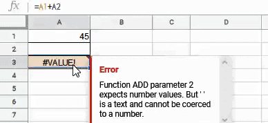
In the image below, cell A2 contains a space, which Google Sheets treats as text. If the cell was blank, the ‘+’ operator would have assumed a value of ‘0’.
Again, since we’re trying to add a numeric value to a text value (‘ ‘), the formula returns a #VALUE! error.
How to Fix the #VALUE! Error
To resolve the #VALUE! error, you can try one of the following:
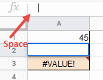
- Look for errant spaces either in your formula or in the cell range specified in the formula. It’s easy to tell if a cell is blank or contains a space character by clicking on the cell. Next, click on the formula bar. You should see a flashing cursor. If there’s a space between the flashing cursor and the character next to it, a space character exists.
2. Check whether any cell in the range contains a text value (even if it looks like a number). You can tell by clicking on the cell and observing how it looks in the formula bar. If you see an apostrophe preceding the value, it’s a text value. Note: You might also get a #VALUE! error if there are spaces inside a date value.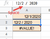
5. #NAME? Error
The #NAME error commonly occurs with formula syntax issues. It could be due to a spelling mistake, an incorrectly named range, or the presence/absence of quotation marks.
If you forget to add quotation marks around a string value, the formula considers it a named range. Furthermore, if a named range by that name doesn’t exist, it returns a #NAME? error.
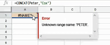
I purposely didn’t put double quotes around the first parameter of the CONCAT function, causing it to consider the first parameter (“Peter”) as a named range. Since it cannot find a named range by that name in the sheet, it returned a #NAME? error.
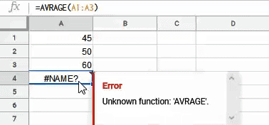
In the next image, I misspelled the function name AVERAGE, causing the formula to return a #NAME? error.
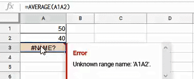
Here, I missed a comma between the cell references A1 and A2. This is a syntax error that results in the AVERAGE function returning a #NAME? error.
How to Fix the #NAME? Error
Since this kind of error is typically related to a syntax issue, check whether there are any spelling mistakes in the function name or named range names.
I also recommend checking whether string values are enclosed in quotations – and that there are both opening and closing quotations for every string value.
If using cell reference ranges, check if you have them separated by a colon symbol. (‘:’).
6. #NUM! Error
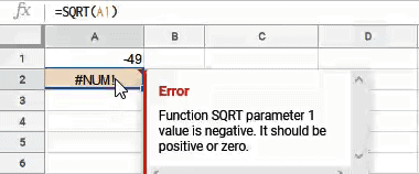
A #NUM error in Google Sheets occurs when a formula has invalid numeric values. Say that you’re trying to find the square root of a negative number, or a calculation results in an enormous number that falls outside the limitations of Google Sheets.
In the image below, we are passing a negative value to the SQRT function (which isn’t acceptable), so the function returns a #NUM! error.
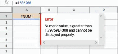
Similarly, I want to find the result of 150 raised to the power of 200, which is a very large number (more than the limit of 1.79769e+308). The formula thus returns a #NUM! error.
How to Fix #NUM Errors
This error means there’s an error with one or more of your numeric arguments. Usually, the error message indicates which issue causes the error. For example, you might spot “Function SQRT parameter 1 value is negative. It should be positive or zero.” In this case, your first parameter in the SQRT function evaluates to a negative number.
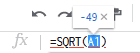
I recommend reevaluating your calculation to ensure that it doesn’t result in a negative number. You can investigate the operation by highlighting – and hovering over – it in the formula bar.
Note: If an operation evaluates to an extremely high number, you won’t be able to see its result in the popup.
#ERROR! Message
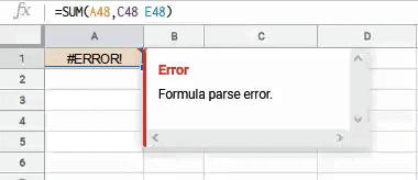
An #ERROR in Google Sheets happens when the program can’t make sense of the formula. More simply, the program doesn’t know what’s wrong with it –– and there could be any number of reasons.
Maybe you forgot to add an important operator between cell references, values, or parameters. In our example, you’d get an #ERROR message if you forgot to add a comma between cell references of non-contiguous cells in your sheet.
It could also happen when your number of opening brackets doesn’t match the number of closing brackets. In the image below, we used a $symbol to refer to a price amount, but Google Sheets mistook it for an absolute reference (making the formula impossible to understand).

This error can also occur if you start text with an equal sign (‘=’). When Google Sheets reads the = sign, it assumes that you’re trying to use a formula.
How to Fix #ERROR in Google Sheets
Resolving this error can sometimes be tough, especially if you have a particularly complex formula. The error message won’t provide any clues about the error, but there are a few steps you can take to resolve the problem:
- Ensure the number of opening and closing brackets match (and that they don’t cause any logical errors).
- Check that colons and commas separate contiguous and non-contiguous cell/range references.
- If using currency or percentage symbols, remove them before applying them to the formula. If you need to use these symbols, enter them as plain numbers (and format the result with an added percentage or currency symbol later).
8. Popup Formula Parse Error in Google Sheets
An error message popup usually occurs when your formula has a fundamental problem. In most cases, you may have accidentally entered a character or symbol in your formula before pressing the return key. It won’t let you alter the formula until you resolve the error.
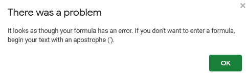
Say that you accidentally entered a backslash character at the end of the formula (before pressing the return key). A mistake like this will most likely result in a formula parse error message popup.
How to Fix the Formula Parse Error Message Popup
It’s best to avoid this error from happening in the first place. Always double-check your formula before hitting the return key.
Make sure there are no surplus characters, missing characters, or wonky cell references.
9. #NULL Error in Google Sheets
There’s no fix for #NULL. It’s only a Microsoft Excel error and doesn’t exist in Google Sheets.
Functions to Help Fix Sheets Formula Parse Errors
There are a few functions that you can use to help identify formula issues and resolve them. Let’s take a look at them and what they do.
=ISNA(value)
Determines whether the cell has an #N/A error
=ISERR(value)
Checks for every other type of error (not including #N/A)
=ERROR.TYPE(value)
Reveals the type of error by returning a number value:
- 1 for #NULL!
- 2 for #DIV/0!
- 3 for #VALUE!
- 4 for #REF!
- 5 for #NAME?
- 6 for #NUM!
- 7 for #N/A
- 8 for all other errors
Google Sheets Formula Pass Error Extra Tips
Sharing with Other Countries
Some international Google Sheets may use semi-colons (;) instead of commas (,). You may want to try swapping those around if you’ve copy-pasted a formula.
Highlighting
If you double-click the cell with the formula, Sheets will usually underline the dysfunctional part of the formula in red. That makes it easier to pick apart your formula.
Formula Parse Error in Google Sheets FAQ
What Does Formula Parse Error Mean?
A formula parse error means you’ve made an error when entering a formula into Google Sheets.
How Do I Remove Formula Parse Error?
Troubleshooting should remove a formula parse error, but several different types of errors can occur. Click the cell to find the type you need to fix, then follow our guide (above) to fix that particular formula parse error.
How Do I Stop Formula Parse Error in Google Sheets?
The most common reason for a formula parse error is a mistyped formula. To minimize them, make sure your syntax and figures are right.
How Do I Get Rid of #DIV 0 in Google Sheets?
The #DIV/0 error occurs when the denominator results in a zero. You can’t divide by zero, so check your formula to determine where this error is coming from.
How Do I Fix the Error Number in Google Sheets?
The #NUM error occurs when the result unexpectedly returns a negative value in a formula that only works with zero or positive numbers. You’ll need to locate the part of your equation that’s causing the negative value result.
Wrapping up
Now that you know how to resolve a formula parse error in Google Sheets, I hope you feel more confident handling the program. If you need more practice, Udacity offers a wide range of courses that are designed to take your skills to the next level.
Related: