How to Use the DATE Google Sheets Function [Easy Examples]

Adding dates to spreadsheets seems like it should be as easy as entering into the cell, right? While that is true most of the time, dates entered in this fashion often cause other functions not to work correctly. It may also cause issues with formatting, i.e., the month before the day is not necessarily the format used in a spreadsheet you import from the web.

To avoid these potential issues, you can use the DATE formula to ensure your dates are formatted correctly as you enter them. Read on to learn how to use the DATE Google Sheets function with detailed examples.

What Is the Google Sheets Date Formula

Dates can sometimes cause issues in spreadsheets. While you can include dates and times in formulas, they often aren’t supported as numerical values. So, you need to make sure the date is surrounded by quotes.

Although Google Sheets has a lot of formulas that allow you to use date and time in their proper formats, the DATE function is the one you should learn first due to its simplicity and the fact that it allows you to use the date as a cell reference for other formulas.

Making sure that Sheets accurately interpret dates, particularly if the input data is not in the relevant format, is an important use for the function. An example of when this could be important is when sorting by date.

The DATE function displays dates that incorporate information from other worksheet places, such as the year, month, or day, to ensure the dates used in the calculation are number format rather than text.

You can also use DATE to create a wide range of date formulas by combining them with various other Google Sheets functions.

Google Sheets DATE Syntax

Before we look at the formula in action, let’s look at the recipe for DATE in Google Sheets and how it works. The syntax for the DATE formula is:

=DATE(year, month, day)

The Google Sheets formula for dates needs three simple parameters to work. These are:

• year: this is the year for the date you wish to enter. Enter this as (yyyy) four-digit format. You can also add the cell reference to the location of the year.
• month: this is the month for the date you wish to enter. Enter this as (mm) two-digit format. You can also add the cell reference to the location of the month.
• day: this is the day for the date you wish to enter. Enter this as (dd) two-digit format. You can also add the cell reference to the location of the day.

Related Reading: Calculate Days Between Dates in Google Sheets

How to Change the Regional Settings

Like many online services, Sheets uses the American dates format by default: MM/DD/YYYY. However, if your region uses a different format, you can adjust Sheets to display the date in your preferred format. You can do this by changing the regional settings.

Follow these steps to change the regional settings for dates in Google Sheets:

1. Click on the File option in the top options bar. This will open a drop-down menu containing a list of options.
2. There, click on Settings to open the menu containing the settings for Sheets. Note that the changes made will only be for that particular spreadsheet,
3. Click on General to go to regional settings for the spreadsheet.
4. Here, click on the box under Locale, which will open a list of the available countries.
5. Click on your country of choice to select it.
6. After you’re done, click the green Save and reload button at the bottom right corner of the box to save the changes and return to your spreadsheet.

From now on, the dates you enter into the spreadsheet will follow the specified formatting of the country you selected. However, you may have to reformat the dates you already have entered into your spreadsheet.

DATE Google Sheets Examples

Now that we know how the function works and its syntax, let’s look at how you can use this function in your spreadsheet.

Simple DATE Sheets Functions

Let’s look at the most basic way of using the DATE formula. Here are the steps you need to follow to do so:

1. Click on a cell you wish to enter the DATE formula.
2. Enter the initial part of the function, which is =DATE(.
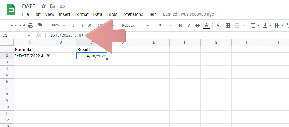
3. Now, enter the first argument parameter, which is the year. In this example, it is 2022.
4. Put a comma ( , ) to divide the parameters.
5. Type in the second argument parameter, which is the month. For this example, we are going to enter 4.
6. Add another comma ( , ) to divide the parameters.
7. Type in the third parameter, which is the day. For this example, we are going to enter 18.
8. Finally, enter a closing bracket “)” to finish the formula.
9. Press the Enter key to execute the formula.

You will see the date displayed in the selected format when the formula executes. Although this may be useful to some, there isn’t much you can do with this formula right now. Let’s look at a few more ways you can use Google spreadsheet DATE formulas.

DATE Formula in Google Sheets With Cell Reference

One useful way you can use the Google Sheets dates formulas is when you have your dates stored in separate cells. Let’s say you have three different cells containing the day, month, and year. You can add a reference to those cells in the DATE formula. Let’s look at the ways you can perform this in your sheet.

Here are the steps you need to follow to use DATE functions in Google Sheets with cell references:

1. Click on a cell you wish to enter the DATE formula.
2. Enter the initial starting part of the function, which is =DATE(.
3. Now, enter the starting parameter, which is the year. In this example, it is cell address C2.
4. Put a comma ( , ) to divide the parameters.
5. Now, type in the second parameter, which is the month. For this example, we are going to enter cell address B2.
6. Add another comma ( , ) to divide the parameters.
7. Now, type in the third parameter, which is the day. For this example, we are going to enter cell address A2.
8. Finally, enter a closing bracket “)” to finish the formula.
9. Press the Enter key to execute the formula.

The benefit of using this method to input dates is that you can dynamically change the dates by making changes to the cell containing the date elements.

Adding Numbers to a Date

Let’s look at another way you can use the DATE formula. In this example, we will add numbers to the date parameters that already exist in a cell. We will use the same parameters from the example above to make it easier to understand. We have the date 04/18/2022, which we wish to convert to 1/1/2030.

To add numbers to the DATE function in Google Sheets, follow these steps:

1. Click on a cell you wish to enter the DATE formula.
2. Enter the initial part of the function, which is =DATE(.
3. Now, enter the first arguement parameter, which is the year. In this example, it is cell address C2.
4. To add the years, type in the plus (+) sign and write 7, which is the number of years we wish to add.
5. Put a comma ( , ) to divide the parameters.
6. Now, type in the second parameter, which is the month. For this example, we are going to enter cell address B2.
7. To add the months, type in the plus (+) sign and write 8, which is the number of months we wish to add.
8. Add another comma ( , ) to divide the parameters.
9. Now, type in the third parameter, which is the day. For this example, we are going to enter cell address A2.
10. To add the days, type in the plus (+) sign and write 14, which is the number of days we wish to add.
11. Finally, enter a closing bracket “)” to finish the formula.
12. Press the Enter key to execute the formula.

Related: How to Use Phone Number Formatting in Google Sheets

Things to Keep in Mind When Using the DATE Function

There are a few things to know when using the formula for dates in Google Sheets. These are:

• Input for the Google Sheet DATE function can not be strings. They need to be entered as numbers. If you add a string in a parameter or reference to a cell containing one, the formula will return a #VALUE! error.
• The Google Sheets DATE function will automatically remove the numerical values after a decimal point. This means that if you enter a value like 11.75, Google Sheets will remove the .75 and interpret the value as 11.
• Sheets uses 1900 as its date system. This means that the oldest date you can enter into Google Sheets is 1/1/1900.
• If you were to use a number below 1900, Sheets will add that value in 1900 to calculate the year. For example, if you write the formula as =DATE(118,1,1), the date will be created as 1/1/2018.
• If you enter the year parameter between 1900 and 9999, Sheets will use the value. For example, if you write the formula as =DATE(2077,1,1), the date will be created as 1/1/2077.
• If you enter the year parameter below 0 or above 9999, Sheets will give you the #NUM! error.
• Google Sheets automatically recalculates days or month parameters outside the valid day and month ranges. For example, if you write the formula as =DATE(2022,13,5), Sheets will recognize the non-existent 13th month and create a date of 1/5/2023. Similarly, if you write the formula which contains an illegal day, such as =DATE(2022,1,32), Sheets will recognize the non-existent 32nd day and create a date of 2/1/2022.

Frequently Asked Questions

How Do You Use the Date Formula in Google Sheets?

The syntax for the DATE formula is =DATE(year, month, day). The formula needs three simple parameters to work. These are the year for the date you wish to enter. The second one is the month for the date you wish to enter. The third parameter is the day for the date you want to enter.

How Can I Quickly Insert a Date in Google Sheets?

The formula is easy to use and doesn’t require you to use any parameters. The syntax for the formula is =NOW(). You can use the NOW function to add the current time and date to your spreadsheet. If you wish to add a specific date, you can use the DATE function. The format for DATE is =DATE(year, month, day).

How Can I Automatically the Fill Cells With Dates?

Click on the cell which contains the first date. Now, drag the thick blue dot towards the bottom of the box to cover the cells you wish to fill with the dates. These fill handles can be dragged in any direction, depending on available space. You may also want to consider adding a date picker to help with frequent date input.

How Can You Format a Date?

To format a date in your spreadsheet, highlight the cell containing the data you wish to edit. Click on Format in the top bar, then click on Number in the drop-down menu. There, click on Custom date and time. In the text box that appears, select a format that you want and then click on Apply.

Wrapping Up The DATE Google Sheets Function Guide

While the DATE Google Sheets formula is helpful for small calculations, you may be better off changing the formatting by selecting the entire row and navigating to Format > Date. In any case, familiarizing yourself with the DATE function is a good call. Let us know in the comments if you have any questions.