Google Sheets is an excellent platform with several features for free to small businesses and individuals, which has caused many people to convert from software like Microsoft Excel.
Many people use spreadsheets to keep track of their finance, grades, or schedules. Some people use Google Sheets for data analysis, which can help understand patterns that allow you to act accordingly. The following article is an in-depth data analysis Google Sheets guide, so read on to learn all about leveraging statistics in your spreadsheets.
This Article Covers:
What Is Google Sheets Data Analysis?
Spreadsheet data analysis is a way to understand and make sense of data but can be complex and intimidating. Often, advanced techniques identify patterns in data and trends that a specific dataset may follow.
A spreadsheet is a great way to lay out your data and keep track of it. For instance, when used in finance, spreadsheets allow you to lay your finances out in an understandable way and calculate your expenses, etc.
But then what? You need data analysis to capitalize on the raw data.
You can analyze your data in Sheets using several methods, including using formulas, using scripts, and creating charts and tables. We will look at some of these methods to help you quickly and easily analyze your data.
Data Analysis Google Sheets Formulas
1) Searching Data in Columns (VLOOKUP)
=VLOOKUP(search-key, range, index, [is-sorted])
This formula can find a specific value in a huge table. All you need to do is enter the exact value and specify the range in which you want to look for the data.
In the VLOOKUP syntax:
- The search-key is the data you wish to find in your table in the formula
- The range defines the cell addresses within which you want to find your data
- The index defines the value you wish to return
- is-sorted identifies whether the column you want to check is sorted or not.
2) Searching for Estimate Data (MATCH and INDEX)
+MATCH(search-key, range, [search-type]) and =INDEX(reference, [row], [column])
Often described as a more dynamic version of the VLOOKUP formula, you can use the MATCH and INDEX in conjunction to search for an estimated value in a spreadsheet, and you can use INDEX to get the address of the cell whose value is defined.
3) Return the Absolute Value of a Number (ABS)
=ABS(value)
You can use this formula to get the absolute values of numbers, and it treats positive and negative numbers as equal. This function is very powerful when used with other functions like SUM, MIN, MAX, and AVERAGE.
4) Finding a UNIQUE Value
=UNIQUE(range)
This formula can help you find uniques values in your data set. To use this formula, all you need to do is write your cell address ranges in the formula, and the UNIQUE function will do the rest of the magic.
5) Counting Cells Meeting a Criteria (COUNTIF)
COUNTIF(range, criteria)
The COUNTIF function essentially allows you to count the cells that meet specific criteria. You can use this formula to count the cells that contain a particular keyword or a value that meets an exact condition.
How to Do Data Analysis in Google Sheets Using Macros
Managing smaller spreadsheets is easy, but having a more extensive spreadsheet that spans multiple pages and has thousands of rows of data can become very cumbersome to manage manually. Using a macro to automate a lot of the work is an excellent option for these data sets.
Macros are user-defined custom functions that can automate your manual tasks. There are virtually no limits to what you can do using a macro. For example, you can increase or change the font of every row using a macro, or you can use macros to convert the currency of every row in your sheets.
This also removes a lot of the tedium of navigating and making changes in a spreadsheet. Making macros work in your spreadsheets is simple. There are essentially two ways to create a macro. You can record a macro, or you can create a script.
Recording a Macro
To record a macro, follow these steps:
Step 1: Click on Extensions in the top bar. There, click on Macros and then click on Record macro
Step 2: As soon as you click on the Record macro, a window will show up at the bottom, showing that the macro is recording. By default, Google Sheets uses Absolute References but feel free to change between them depending on your needs. Once you record your actions, simply click on Save.

Step 3: Select a name for your macro, and you can also set up a shortcut key to allow you to access the macro easily.

There are two types of referencing models used in Google Sheets, Absolute, and Relative:
- Absolute Reference works for that exact cell you edit, so it will edit the same cell every time you execute the macro. This is much more useful for setting up things like headers and title cells.
- Relative Reference adjusts the macro according to your cursor. For example, if you recorded the macro to change the properties of the cell five steps to the right, then the macro will change cell D5 if you select D1 and, in a similar fashion, B10 if you select B5 and so on.
How to Analyze Data in Google Sheets Using a Script
You can use Apps Script, a scripting tool built into Google Sheets, to set up a macro. To do this:
Step 1: On the main screen in Sheets, click on Extensions in the top bar and click on Apps Script. This opens the Apps Script editor on a new page.

Step 2: Start to write the macro function. Note that they don’t take any arguments and don’t return any values.
Step 3: Edit your script manifest to make the macro and link that to the macro function. You can also assign a name and a keyboard shortcut to your macro.
Step 4: Save the script project, and the macro should be available for use in your sheet.
Step 5: Test your macro to ensure it works properly.
Scripts can be pretty complicated and intimidating to new users, so check out our Scripts guide here if you’re a little confused.
Google Sheets Analytics With Tables and Charts
Using tables and charts can be a great way to visualize your data presentably. Here are the steps you need to follow to create a chart on Google Sheets:
Step 1: Click on Insert in the top bar and click on Chart. You will see a blank chart appear on the screen.

Step 2: To create the chart, you need to enter the cell range. To do this, simply write the addresses in the Data Range textbox. As soon as you press enter, the chart should appear. You can choose to change the visual elements in your chart by going to the Customise tab.

Step 3: Click on the chart, and you will see a blue border around it signifying that it’s selected. You can move it around or resize it by selecting and dragging any of the 8 blue dots. You can also click on the three dots on the top right to edit the chart or download it.

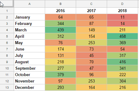
Use Conditional Formatting to Visualize Data
Conditional formatting makes your data much easier to view and to extract relevant data for analysis. You can highlight cells that meet conditions with different colors or other visual preferences. To do this, follow these steps:
Step 1: Select the cells to which you want to apply the conditional formatting. Select Format from the top bar and then click on Conditional Formatting. A sidebar will show up on the screen that allows you to set the conditions.

Step 2: In the sidebar, first write the cell range to apply the changes in the Apply to range text box. You don’t have to worry about this if you have already selected the cells in step 1. Next apply formatting rules under the Format rules option. In this particular case, we set up conditional formatting to only turn those cells with a value of more than $200,000,000 green.

Step 3: Once you’re done with the setup, simply click on Done to save the changes. If you wish to make multiple rules, click on Add another rule and repeat the same steps.

There is virtually no limit to how many rules you can add to your spreadsheet.
Use a Google Sheets Statistics Add-on
If you need to do statistical analysis, the easiest way to do so is often through an add-on package like Statistical Analysis Tools (follow the link to download and apply it to your browser). Then to use it, just navigate to Add-on > Statistical analysis tools.
There are too many functions to give a detailed guide for each here, but the interface is very intuitive and can help with analysis types including:
- Exponential smoothing
- Moving average
- Correlation
- Covariance
And much more, along the lines of Regression Analysis in Google Sheets, etc.
Several other add-ons are great for data analysis. Some of our favorites are:
Frequently Asked Questions
Does Google Sheets Have Data Analysis?
Google Sheets has some tools built in that allow you to analyze data and get some useful insights. These include charts, tables, and conditional formatting that allow you to do data analysis. You can also use add-ons for more types of data analysis.
What Is Analysis Google in Sheets?
Spreadsheets are a great way to organize your data. But, figuring out what to do with the data is another story. Analysis helps you or your business interpret raw data and make informed decisions about it.
What Features Can You Use in Google Sheets to Analyze Data Efficiently?
You can apply conditional formatting to color-code your data, use pivot tables and funnel charts to show the flow of data and visualize it, and use macros to automate a lot of your tasks.
Get Analyzing
Now that you understand data analysis Google Sheets formulas and functions, all that’s left to do is apply what you’ve learned in your spreadsheets. If you’d like to learn more about Google Sheets, a good next step is to learn how to validate data in Google Sheets.
Related: