
If you’re creating a timetable for students in Google Sheets, or just planning ahead, you may need to know when is the last Monday of the month (or any other last weekday day of the month). To calculate this, you can simply use the Google Sheets EOMONTH function
In this tutorial, I will show you how to use formulas in Google Sheets to do this.
Use the Google Sheets EOMONTH Formula to Calculate the Last Monday of the Month
Suppose you want to know what would be the date of the last Monday in the month of June 2018.
Below is the EOMONTH function that will give you the month and date in Google Sheets:
=EOMONTH(DATE(2018,5,1),0)-WEEKDAY(EOMONTH(DATE(2018,5,1),0),2)+1
How does the formula work?
There are 3 Google Sheets functions that are used to calculate this:
- EOMONTH: This function finds the last date of a given month. It stands for ‘End Of Month’ and is the among the most commonly used MONTH formulas is Google Sheets
- WEEKDAY: This function tells us the weekday number of a given date. In this example, the last date of June 2018 was 30/6/2018 which was a Saturday. So Weekday function gave us 6 for Saturday (the numbering started from Monday. So Monday is 1, Tuesday is 2, and so on).
- DATE: This function gives us the date when we specify the year, month and day value.
Now let me try and break it down further:
EOMONTH(DATE(2018,5,1),0)
This part of the formula would give us the last date in June 2018. Note that I have used ‘0’ as the second argument (which makes google Sheets provide the end of month date in which the first argument belongs).
You can also use this function to get the last date of the previous/next month (instead of 0 use 1 for next month and -1 for the previous month).
WEEKDAY(EOMONTH(DATE(2018,5,1),0),2)
The above part of the formula tells us what weekday is the last day of the month. In this example, this will return 6, as the last day of the week is Saturday.
=EOMONTH(DATE(2018,5,1),0)-WEEKDAY(EOMONTH(DATE(2018,5,1),0),2)+1
Finally, this formula gives us the last Monday of the month.
You can also use this same technique to calculate any day of the month. For example, if you want to know the third Thursday in June 2018, you can use the below formula:
=EOMONTH(DATE(2018,6,1),-1)+1+IF(WEEKDAY(EOMONTH(DATE(2018,6,1),-1)+1,2)>4,4-WEEKDAY(EOMONTH(DATE(2018,6,1),-1)+1,2)+7,4-WEEKDAY(EOMONTH(DATE(2018,6,1),-1)+1,2))+7*2
This technique can also be used to calculate holidays in a year. For example, if you want to know the date of Labor Day, which is first Monday in September, then you can use this technique.
Use Case Example – Using EOMONTH to Calculate Employee Benefits
As employee bonuses and benefits often begin after a certain number of full months after joining the team, the EOMONTH Google Sheets function is a good way to calculate exactly when an employee becomes eligible. Take a look at the following example:
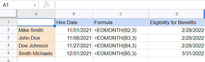
As you can see “Smith Michaels” has a different employee benefit date than “Doe Johnson” even though he was only employed a few days after the latter.
You May Also Like the Following Google Sheets Tutorials: