
You can calculate weighted averages in Google Sheets by using a built-in formula: AVERAGE.WEIGHTED.
Weighted averages are useful for calculating average scores when some factors are more important than others.
What is weighted average? A weighted average is similar to an average of numbers, but each number makes up a different share of the average.
For example, you may have a class where there are two tests worth a different portion of your grade: the midterm is 40 percent while the final is 60 percent.
The AVERAGE.WEIGHTED function expands on the AVERAGE function.
Additionally, Google Sheets and Microsoft Excel both support a similar function called SUMPRODUCT, but the AVERAGE.WEIGHTED function can return the results you’re looking for with less effort in most cases.
The following processes will teach you how to calculate weighted average using the AVERAGE.WEIGHTED function in Google Sheets.
This Article Covers:
Calculate Weighted Average In Google Sheets using Percentage Weights
The weighted average formula in Google Sheets uses two data set inputs:
- the values and
- the weights
Below is the syntax of the Average.Weighted function:
=AVERAGE.WEIGHTED(values, weights)
When you’ve added values, it will look something like:
=AVERAGE.WEIGHTED(A1:A5,B1:B5)
We’ll look at how this function works with the following class grades dataset.
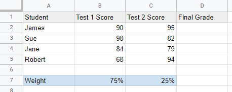
The class featured two tests making up 75 and 25 percent of the final grade respectively. The example uses percent values to establish the weighting.
The following steps explain how to calculate the weighted average in Google Sheets:
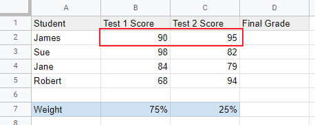
- Determine the “values” criteria for the formula. In this case, we’ll be combining the values in columns B and C for the students, so our value will be “B2:C2” for the formula in cell D2. It will grab from the same row B and C cells when expanded to the rest of column D.

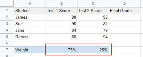
- Determine the “weighted” criteria for the formula. In our example, the weight values are stored in cells B7 and C7. Since we don’t want these values to change, we need to set them to static values, so our weighted criteria will be “$B$7:$C$7.” In the example, we are using “%” scores to assign weights.
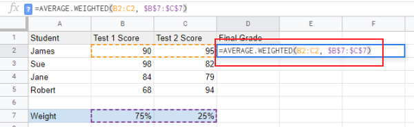
- Add the criteria to the formula =AVERAGE.WEIGHTED(values, weights). The example formula is
=AVERAGE.WEIGHTED(B2:C2, $B$7:$C$7)
- Enter the formula in the topmost cell for the return values column. The example shows adding the formula to cell D2.

- This will return the results for cell D2; drag the bottom right icon in the cell for the rest of the rows to apply the formula across the spreadsheet.

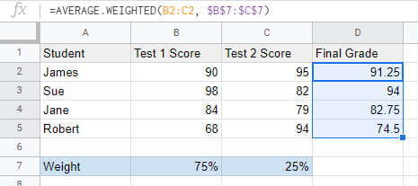
The formula will return the weighted averages. With James, the formula is calculating =SUM((B2*0.75)+(C2*0.25)), but uses a syntax that will update for all cells if you change the weighted value.
Additionally, manually building weighted calculations can get very cumbersome if you have more than a few values to average.
Calculate Weighted Average in Google Sheets with Quantity Weights
The convenience of knowing how much each value in the average will be weighted by a percentage is a luxury you don’t get in a lot of cases.
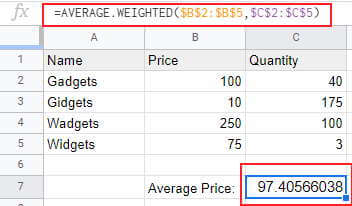
In this example, we’ll determine the average selling price of a product at a hypothetical store. Column A has the product names, Column B has the selling price, and Column C contains the quantity sold.
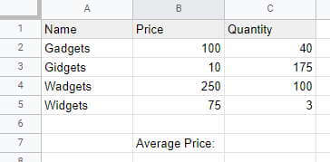
Unlike the previous example, this one doesn’t use a percentage value to determine weight. Instead, the formula will calculate the weight percentages automatically based on the sum of the values.
In this version, the price is the value, but the quantity sold values are the weights.
Follow these steps to use the WEIGHTED.AVERAGE formula to calculate the average selling price
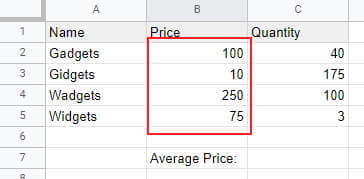
- Determine the “values” criteria for the formula. In this case, we’ll be combining the values in column B. We don’t want these values to change, so the example value criteria are: “$B$2:$B$5”

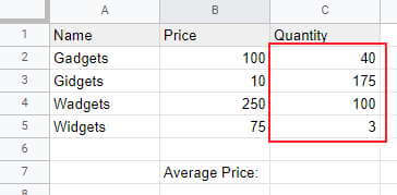
- Determine the “weighted” criteria for the formula. In our example, the weight values are stored in column C. We don’t want these values to change, so the example weighted criteria are: “$C$2:$C$5”
- Add the criteria to the formula =AVERAGE.WEIGHTED(values, weights). The example formula is
=AVERAGE.WEIGHTED($B$2:$B$5,$C$2:$C$5)
- Enter the formula in the return cell to run the function. In the example, the formula returns a rounded value of “94.4.

Calculate Weighted Average in Google Sheets with Additional Values
You can expand on how the =AVERAGE.WEIGHTED function works by adding additional values. This feature is useful if you need to add weighted values outside of the predetermined range.
For example, a teacher might throw some students a freebie with their grades by adding an additional weighted assignment with a perfect score to the grade calculation.
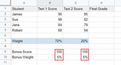
For this example, we’ll use the same grades from the first example, except we’ll change the weight values and add two “perfect score” bonus assignments for all students.
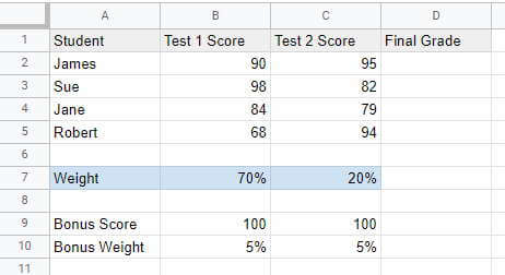
The appended formula looks like this:
=AVERAGE.WEIGHTED(values, weights, [additional values], [additional weights])
When filled out with one additional value it looks like this:
=AVERAGE.WEIGHTED(A1:A5, B1:B5, C5, D5)
When filled out with two additional values it looks like this:
=AVERAGE.WEIGHTED(A1:A5, B1:B5, C5, D5, C6, D6)
Notice that the formula uses the pattern “additional value 1, additional weight 1, additional value 2, additional weight 2.” It goes “value, weight” repeat as opposed to “all values, all weights.”
Follow these steps to calculate the weighted average with additional weights:
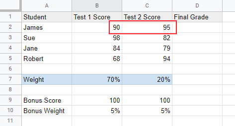
- Determine the “values” criteria for the formula. In this case, we’ll be combining the values in columns B and C for the students, so our value will be “B2:C2” for the formula in cell D2. It will grab from the same row B and C cells when expanded to the rest of column D.
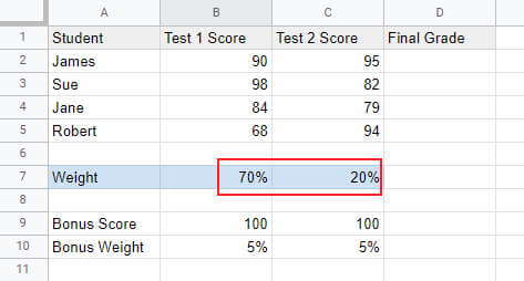
- Determine the “weighted” criteria for the formula. In our example, the weight values are stored in cells B7 and C7. Since we don’t want these values to change, we need to set them to static values, so our weighted criteria will be “$B$7:$C$7.”

- Determine the “additional values” and “additional weights” criteria for the formula. In this example, we’re bringing in additional values from cells B9 and C9, with their corresponding weights in cells B10 and C10. This is expressed as “$B$9,$B$10,$C$9,$C$10.”
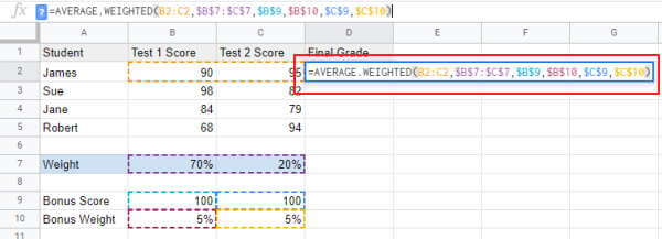
- Add the criteria to the formula =AVERAGE.WEIGHTED(values, weights, [additional values], [additional weights]). The example formula is
=AVERAGE.WEIGHTED(B2:C2,$B$7:$C$7,$B$9,$B$10,$C$9,$C$10).
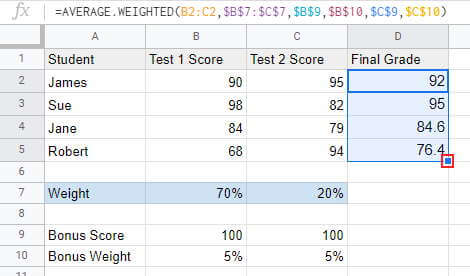
- Enter the formula in the topmost cell for the return values column. The example shows adding the formula to cell D2.

- This will return the results for cell D2; drag the bottom right icon in the cell for the rest of the rows to apply the formula across the spreadsheet.

The average weighted formula can substantially cut down on the amount of work you need to do in Google Sheets to calculate weighted averages.
I hope you found this tutorial useful!
Other Google Sheets tutorials you may like: