How to Make Google Sheets Run Macro Automatically

Speeding up your spreadsheet work by automating tasks has never been this easy, thanks to macros. Google Sheets allows you to record macros. These are a series of steps that you can automate, so you won’t need to do the same things in the spreadsheet over and over again, saving you time in your work.

The uses for Google Sheets to run macro automatically include formatting data, adjusting the font style and size, adjusting indents, adding rows or columns, or any action in the software. Macros even let you link a customized keyboard shortcut and execute it to another data set in the spreadsheet just by using your keyboard.

Macros save automatically to the spreadsheet you are working on, so the next time you need to apply the same formatting to another data set, just click the macro you created before. In just a matter of seconds, your sheet will look precisely like what you want it to.

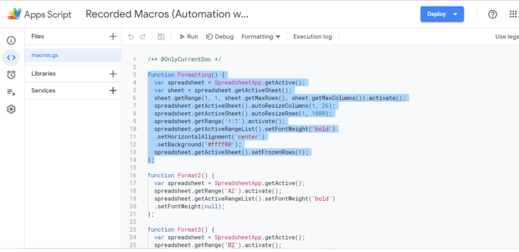
Macro functions are generated in the Apps Script function, also known as the macro function, of Google Sheets.

It is bound to a script project with the title “macros.gs”.

You can use the Apps Script to write and create macros. But if you don’t know how to write codes, you can simply follow these steps in creating macros.

Creating a Macro in Google Sheets

Below are some Google Sheets script examples of spreadsheets with long lists of data.

Say you’re tasked to format it to make it look organized. You may want to make the rows and columns be of the same size, make sure that you can see all the texts in the cells, make the headings bold and highlighted in yellow, and freeze the first row so that you can easily navigate the remaining data at the bottom of the spreadsheet.

That’s a lot of functions, right? Macros can help make this easier to do continuously.

The first thing you need to do is Go to Tools > Macros > Record Macro.

After that, you’ll be prompted to record a macro. You’ll see ‘Recording new macro…’ at the bottom of the spreadsheet too.

You will then have two options: ‘Use Absolute references’ or ‘Use relative references.’

• Using absolute references allows the macro to apply the action to the same cell, row, or column you click. For example, if you make cell B1 bold, the macro will always make cell B1 bold.
• Setting it to relative references will let the macro apply the formatting to the cell you selected. If you make cell B1 italicized, the macro will make any relative cell to it, say C1 or D1, italicized, too.

For this example, we will use absolute references.

Once your macro is set to record, you can start modifying your spreadsheet.

Record the first action you want to make. In this case, we will make the rows and columns the same size and all text in the cells visible. To do this;

1. Select all the data in the spreadsheet by left-clicking the uppermost and leftmost cell on the spreadsheet.
2. Once you’ve selected all the data, double-click on the column separator of any cell, then on the row separator. You will see that the spreadsheet looks better now.
   
   If you look at the bottom information in your spreadsheet, ‘Recording new macro…’, you will see that every action you make appears on the box. In this case, it showed ‘Action 3: Auto resize rows’, which I did to make the rows of the same size. You can use this information to double-check your work or check if you employed the correct action to the spreadsheet.
3. Next is to make the headings of the data bold and highlighted in yellow. Click on cell 1:1 to select all the titles automatically in the spreadsheet, press ‘Ctrl + B’ or the ‘B’ button at the top to make the letters bold, then click on ‘Fill Color’ and select the color yellow to highlight the texts. After that, your spreadsheet will look like this.
   
4. Lastly, go to View > Freeze > 1 row. This action will freeze the data up to the first row so that the first row (the heading) will always be visible when you scroll down.
5. After performing all the actions, you need to automate in the spreadsheet, click on ‘Save’ to save your macro.
   
6. Type the name you want for your macro into the box that will appear on your screen. In this case, I wrote ‘Formatting.’ You can also create a keyboard shortcut with the form ‘Ctrl + Alt + Shift + Number.’ This will make it easier for you to execute the macro in another sheet of the spreadsheet. Click on ‘Save’ to save your macro.

The next time you’re given a spreadsheet like this one, you won’t have to perform all the actions again to achieve the desired format. Just click on Tools > Macros > ‘Formatting’ (the macro’s name you created).

You can also press ‘Ctrl + Alt + Shift + 1’ (the number you assigned your macro to). To add another macro in your spreadsheet, just repeat the process above. Click on Tools > Macros > Record macro and start performing the actions you want to be recorded to make another format.

Be sure to write another name for your macro so that you won’t be confused. Don’t forget to input the keyboard shortcut to make executing the macro easier.

You can add up to 10 macros into a spreadsheet.

If you want to edit the name and keyboard shortcut of the macro you created, just:

1. Click on Tools > Macros > Manage macros. A box will show on your screen, containing the names and keyboard shortcuts of the macros you created.
2. Type in the new name you want for your macro or edit the number shortcut
3.  Click on ‘Update’

Editing Using Google Sheets Macro language

You can edit the macros attached to a spreadsheet if ever there’s something you want to change. To edit a macro:

1. Click on Tools > Macros > Manage macros and select the macro you want to edit.
2. Click on the three-dotted lines beside the macro, then select ‘Edit Script.’
3. Sheets will direct you to the Apps Script editor of the Google Sheets, which contains the macro functions of the macros you created. Edit the specific action you want to change in the macro function.
4. Save the script project by pressing ‘Ctrl + S,’ check if the macro function you edited does the action relative to changes you made.

Importing Macros to Another Spreadsheet

You can only apply the macros you created to the same spreadsheet you built them on, and you cannot use it to execute the automation to another spreadsheet. Fortunately, you can import macros to another spreadsheet.

To import a macro:

1. Open the Google Sheet that contains the macro, click on Tools > Macros > Manage macros.
2. Click the three dots beside the macro and select ‘Edit Script.’ The Apps Script of Google Sheets will show on your window. You will find that all the macros you made are contained in the script project.
3. To import the macro, highlight the code of the macro function containing your desired macro. For this example, I’ll import the macro we created earlier entitled “Formatting.”
4. Make sure that you have selected the code up to the semicolon for the macro to work correctly.”. Press ‘Ctrl + C’ to copy it.
5. Open the other spreadsheet where you want the macro imported. In that spreadsheet, click on Tools > Macros > Record macro.
6. You will need to create a macro in this spreadsheet for you to be able to generate a script editor. However, you don’t have to perform any actions on the spreadsheet after recording. Just click ‘Save’ on the box that will appear and input a name for your macro. I named this macro “Formatting (Imported)”. Click on ‘Save’ to save your macro.
7. Open the script editor of your new spreadsheet by clicking on Tools > Macros > Manage macros. Click the three dots beside the macro and select ‘Edit Script’. Once you’re in the Apps Script, highlight the function in the script project and press ‘Delete.’
8. Paste the code that you have copied earlier from the macro function in the original spreadsheet. Press ‘Ctrl + S’ to save the script project.
9. Go back to the spreadsheet and click on Tools > Macros > Import. A box similar to the one below will appear on your screen. Click on ‘Add Function’ under the macro.
10. After adding the function, you will see that a checkmark will replace it. The macro is now added to your new spreadsheet.

However, the macro is not assigned with a keyboard shortcut. You may want to give a shortcut for easier access. To do this, click on Tools > Macros > Manage macros, assign a number you want for the macro, and click ‘Update.’ The macro in your new spreadsheet now has a keyboard shortcut.

To check if your imported macro is working, click on Tools > Macros > “Formatting” or press ‘Ctrl + Alt + Shift + 1’. The spreadsheet should now look like your previous spreadsheet.

Some Things to Keep In Mind When Using Google Sheets Macros

When given a new spreadsheet, maximize the use of your macros by just copying the sheet to the original spreadsheet containing your macros or making a copy of that Sheet. Through this, you won’t have to do repetitive actions in Google Sheets manually.

You can record lots of actions using a single macro. However, macros do well if registered with limited actions. If you have numerous formatting requirements in a single sheet, it’s better to make multiple macros. Just make sure to assign a unique keyboard shortcut to every macro you make, and remember that you can only make up to 10 macros in a spreadsheet.

Can You Run Excel Macros in Google Sheets?

Macros you make in Sheets, unfortunately, are only applicable to Google Sheets. You cannot copy or create macros in other Google Suite tools, and it’s also not easy to import Excel macro to Google Sheets or covert them.

Moving Forward With Macros

Macros may take a while to wrap your head around how to run a Google Sheets macro automatically, but it will save you so much time in the long run. Automation cuts working time down drastically.

Check out our other Google Sheets guides to help you become the best spreadsheet user you can be.