Free Google Sheets Attendance Template – Easy to Use in 2024

Attendance sheets are used in a number of industries and organizations to keep a record of the turnout, and for effective attendance management. In schools and colleges, teachers use attendance sheets to make sure students attend classes regularly and to detect problems in case of anomalies in a student’s attendance.

Besides the education industry, attendance sheets are also used in companies to track employee attendance and consolidate information for ACRs, salary payment, etc.

Gone are the days when you manually had to enter attendance in a big register and then count them out at the end of the month. With modern spreadsheet software, keeping track of attendance is quick and easy.

Moreover, it automates the process, so once you have an attendance template ready with all the required formulae, you can re-use it every month, without having to re-do calculations each time.

In this tutorial, we will show you how to make a simple Google Sheets attendance template, using some simple Google Sheets formulae.

What Does an Attendance Template Consist of?

An attendance template or Attendance tracker in Google Sheets, consists of a grid where details about attendance of a group of people are recorded. Here the group of people may consist of students in a class, employees in a department, or guests at an event.

Other details such as class, group, or department name, and in some cases, time and date may also be recorded in the attendance sheet.

How to Create a Google Sheets Attendance Template

To create an attendance spreadsheet, we start by creating a basic skeleton, or outline of the sheet, in which we create slots for days in the month, student names, and other basic details such as Class / Department / Group, names, dates, etc.

We also put basic conditional formatting into place to highlight weekend days in a different background color or font. This will ensure that attendance entries are not entered into the weekend slots by mistake.

Once the basic skeleton is ready, we can start filling in the basic details such as names, date, etc. We will also put formulae in place to count the number of present, absent, and other types of initials. At this point, we can also add a function to calculate the attendance percentage for each person.

Once the sheet is ready, we can start filling in the attendance grid with the appropriate code for each student on each day of the month.

In this tutorial, we will show you step by step how to create attendance sheets. This attendance sheet will automatically count the number of days present and absent for the entire term.

Download the Free Google Sheets Attendance Template

Using the Free Google Sheets Attendance Template

This template is set up to accommodate a standard 10, or 11-week term. You can also add to that if you want to use the same spreadsheet for the entire year, or delete unused weeks if you only need the attendance template for a shorter period. We’ll show you how to do this later in this article.

Our template provides a weekly roll on each sheet that automatically updates the date range based on the input from the first sheet. We highlighted the date in red to make it easy to see exactly where to put the starting date in the first sheet.

You simply have to double click here, and a calendar will pop up for you to select the current date. The days of the week and date will automatically update in each subsequent sheet.

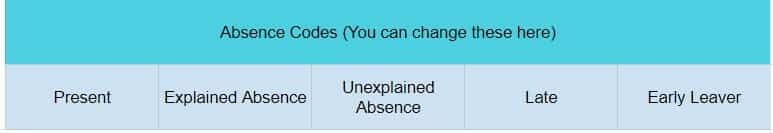
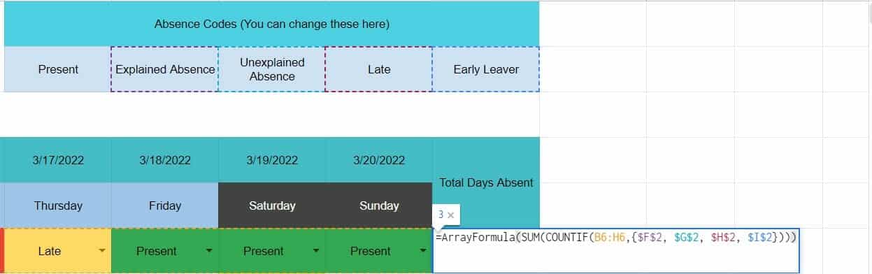
Editing the Codes

There are 5 default input codes you can use in your attendance sheet. Changing the text in the box at the top of the sheet will change what shows up in the drop-down boxes in the main part of the template. Again, you only have to make the changes in the first sheet, and it will apply to all subsequent weeks in the template.

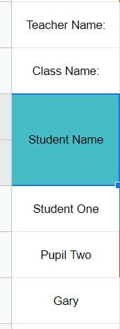
Naming Cells and Ranges

As the default settings for this template is for a classroom, there are cells for you to enter the teacher name, class name, and student names. The spreadsheet will also automatically fill the names into every week. If you work in a different industry, you can simply change the text in Week 1, and all subsequent weeks will match the changes you made.

Using the Dropdown Boxes

The template has a dropdown menu for each student on every day of the week. You have to click the small arrow in the box and make a selection.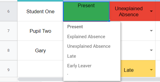

You will notice that one of the options is a single quotation mark. Select this if you want to make the cell blank again.

Each of the choices in the menu will conditionally format the cell to:

• Green – Present
• Yellow – Partially absent (Late, Early Leaver)
• Red – Absent (Unexplained Absence, Explained Absence)

This is to make it easy to see at a glance who has had poor or excellent attendance throughout the week.

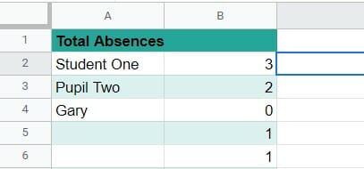
Total Days Absent

The last column in the template calculates how many days a person was absent during the week. It includes partial absences, so be aware of that when making judgments. The last sheet in the template also tracks the total absences throughout the term by adding the values from every week.

How Does the Attendance Template Work?

If you’d like to make any serious changes to the template or build your own, it’s important to understand the concepts we used to put the spreadsheet together. So, let’s take a look at the functions and formulas in this spreadsheet.

Building Automatically Updating Dates

As you’ve probably worked out by now, the rest of the dates in each sheet automatically update based on the date you put into cell B1. To make this happen, we just used cell references and simple addition.

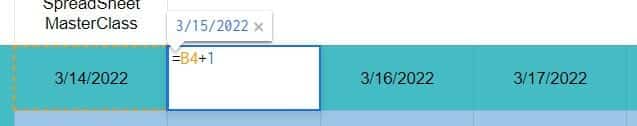
The first cell to have a date in for the purpose of attendance marking is B4, and since this is the same as the starting date, we just had to make it show the same date as the date in B1. So, we simply used the formula =B1.

For subsequent days, we just had to add a day to the previous one. So the cell for Tuesday in the following screenshot just had to have =B4+1, Wednesday has =C4+1, Etc.

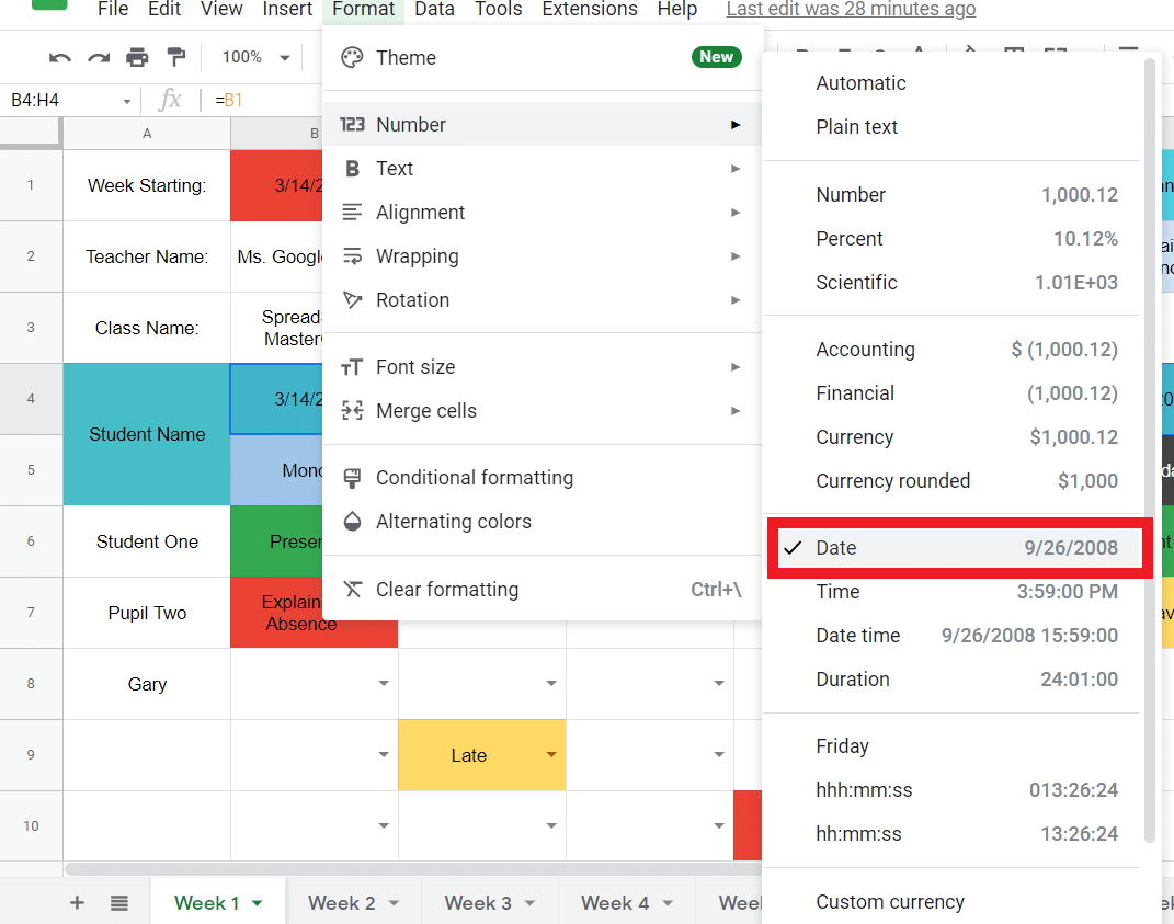
However, to make sure the cells display a date after using a formula, you must ensure the cells are formatted for dates. To do this:

1. Highlight the cells
2. Navigate to Format > Number >Date

Note: You can also change the date format by navigating to Format > Number >Custom Date and Time. This can be handy if you want to display the day before the month.

Displaying the Correct Day of the Week

Underneath each date is the day of the week that date falls on. This stays consistent no matter what. For example, if you entered a Wednesday into the B2 “Week Starting” cell. Then the first day would change to a Wednesday like so:

To make this happen, we just used cell references and formatting again. Each day pulls the data from the date above it. Cell B5 has =B4 as its formula, C5 has =C4, etc.

Initially, it will just display the date a second time when you do this. To change it to the day:

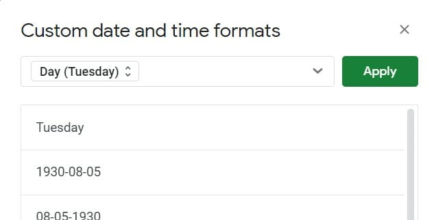
1. Navigate to Format > Number >Custom Date and Time
2. In the menu that pops up, remove anything that is currently in the dropdown box
3. There should be a day of the week in the options below. Click on that.
4. Click Apply

Building the Dropdown Boxes

You can build dropdown menus with a Google Sheets feature known as data validation. This feature works by only allowing certain inputs into cells, hence why a dropdown box then makes suitable inputs as it’s a way of limiting what users can place in the cell.

The first step to using data validation is to define suitable inputs. In the case of our spreadsheet, we have:

• Present
• Explained Absence
• Unexplained Absence
• Late
• Early Leaver
• , (hidden)

These options take up cells E2 to J2.

To use these as references for the drop-down boxes, all you have to do is:

1. Highlight the relevant cells
2. Navigate to Data > Data validation
3. Select List from a range under the Criteria option
4. Define the range you want to use as options in the dropdown menu. In our case, it’s=$D$2:$J$2
5. Click Show dropdown list in cell
6. Click Save

If you don’t want any other inputs to go into the cells, you can check Reject input.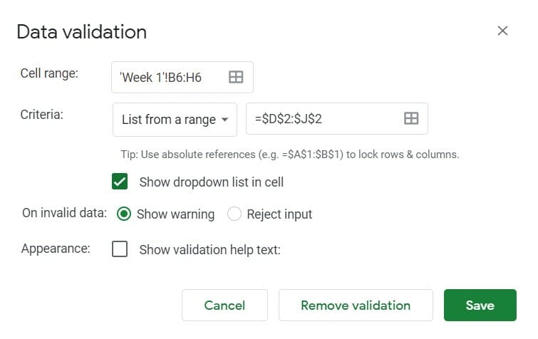

Note: Make sure you use absolute references (with a $ in front), so when you click and drag to apply the data validation to other cells the formula doesn’t change. For example, if you just put D2:J2, when you use the data validation one row down, it will be looking in cells D3:J3 where there aren’t correct options to apply.

Adding Conditional Formatting

Each choice in the dropdown menu will conditionally format the cell to a certain color. This is quite simple to do. Just use the following steps:

1. Highlight the cells you want to apply the conditional formatting to
2. Navigate to Format > Conditional formatting
3. Select the Format rule and define it (Text is exactly Present in the example)
4. Choose the formatting style (we chose a green fill in the example)
5. Click + Add another rule and repeat for all options
6. Click Done

Calculating Total Days Absent

To calculate the total days a person was absent in a week, we used the following formula:

=ArrayFormula(SUM(COUNTIF(B6:H6,{$F$2, $G$2, $H$2, $I$2})))

You’ll notice here that we used absolute references again. These references point to:

• • Explained Absence
  • Unexplained Absence
  • Late
  • Early Leaver

Once again, you must use absolute values so the formula doesn’t break when applied to other rows.

The COUNTIF formula will then look at the defined range of B6:H6, search for those values, and count each one when it appears.

Unfortunately, the COUNTIF function can only search and count one value when used independently. That’s why the above formula has the SUM function to add them together and the ARRAYFORMULA to allow for a search of more than one value.

Referencing Other Sheets

As this spreadsheet template is spread out across several sheets, there are many instances where each sheet needs to pull data from another. One example is the student names. Without automatically moving the data to the next sheet, you would have to manually enter the names every week.

Here’s an example:

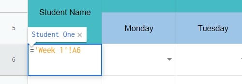
You can see that the cell pulls the name “Student One” from cell A6 in the sheet Week 1.

When using this type of cell reference, make sure the sheet name is enclosed in single quotation marks, and there is an exclamation mark before the cell reference. Otherwise, Google Sheets may try to pull the data from the same sheet, resulting in an error.

You can also make formulas by bringing over data from other sheets. A simple example of this is getting the dates into each sheet. From Week 2 onwards, the starting date used the formula:

=’Week X’ !B1 + 7

X is the previous week.

This is how the spreadsheet automatically updates each week to have to correct dates based on a single input.

Related: How to make a Google Sheets Dependent Drop Down List

Changes You Can Make to the Template

After reviewing the formulas and functions, we used to build the sheet, hopefully, you feel comfortable editing the template to meet your needs.

The standard changes you should make are:

• Defining the start date
• Choosing absence codes
• Filling in student names

Some others you may not have thought of include:

• Changing the conditional formatting of the dropdown menus. For example, you may want different colors for explained and unexplained absences.
• Editing the Total day absent formula to not include the partial absences. (Just get rid of the cell references $H$2 and $I$2) <>Add more weeks to the template. To do this:
  • Right-click on Week 11 at the bottom of the sheet
  • Click Duplicate
  • Rename the new duplicate to Week 12
  • Change the formula in cell B1 to =’Week 11’ !B1 + 7 (or manually enter the date)

Start Using the Template

The sheet has no restrictions, so feel free to make a copy of our free Google Sheets attendance template and mess around with it. If you have any further questions about using it or changes you can make, just ask in the comments!