If you’re new to Google Sheets or you’ve never relied on the “hide rows” feature, you may be a little confused looking at a workbook where rows are missing from the display.
Hiding rows in Google Sheets is very helpful for showing off the data you want someone to look at in a spreadsheet. Google Sheets offers a few ways to unhide rows in a spreadsheet.
However, if you are trying to look at all the data in a spreadsheet, you need to unhide the data found in hidden rows. So how do you unhide rows in Google Sheets?
This tutorial shows you how to unhide rows in Google Sheets in a few different ways. Let’s get started!
This Article Covers:
Note: All these methods also work for hidden columns.
Method 1: Unhide Rows by Clicking the Up/Down Caret Icon
Sheets displays upward, and downward-facing caret icons on the rows above and below hidden row ranges, if you are wondering how to unhide a row in Google Sheets, you simply have to click them.
The following spreadsheet hides rows 4 through 6. You can tell those rows are missing because the numbering jumps from 3 to 7 and there are up/down caret icons next to the range.
If you left-click on either of the caret icons, Google Sheets will show the data in the hidden rows again. This is also how to view hidden rows in Google Sheets for people who are sharing the file with the owner.
The below image shows how Google Sheets will automatically select the data in the formerly hidden row range.

Method 2: How to Unhide Rows in a Selection Range
Clicking the icons is straightforward and shows individually hidden row groupings. However, you may encounter more complicated use cases where you want to unhide multiple row groups or all the rows on a page in order to unhide cells in Google Sheets. In this case, there is another method in Google Sheets that can show how to unhide rows.
In the following example, Google Sheets hides nonconsecutive rows in two groups.

We can’t see the information in rows 4, 5, 8, and 9. The hidden rows are designated by the caret icons above and below the neighboring row numbers. The process of unhiding two or more groups of hidden rows is the same. This is useful if you want to manipulate every other row.
The following steps demonstrate how to unhide multiple hidden row groupings simultaneously.
- Highlight the desired range of rows you want to show. Manually select the range by left-clicking a row above the first hidden group. Then hold the “shift” key and select a row below the hidden group range.

- The example shows clicking on rows 3 and 10. This will highlight the entire range of hidden rows. Alternatively, you can select the entire sheet if you want to Ctrl+A on Windows/ChromeOS or Command+A on MacOS.

- Right-click somewhere within the selected range and choose“Unhide rows” from the menu. Alternatively, you can use the keyboard shortcut Ctrl+Shift+9 on Windows/ChromeOS or Cmd+Shift+9 on MacOS.


Google Sheets will now show and select all the rows within the formerly hidden range.

Method 3: Set Groups to Hide and Unhide Google Sheets Rows Fast
There is a built-in feature fora Google spreadsheet to unhide rows for easily that doesn’t go away when you choose to unhide data. This feature works well with multiple rows. The “group” function assigns a “+/-” icon to a row range that toggles show/hide functionality.
You may encounter workbooks already using “group” to hide data. The following example shows two hidden groups designed by a “+” icon to the left of the hidden row range.
Just left-click on the icon to show the hidden rows. If you’re working on a shared spreadsheet, adding group-based hiding is a great way to preserve the hidden row feature someone else added to the sheet while still being able to view content in hidden rows.
Assigning a group is a straightforward process.
- Select the rows you want to group by clicking the first row and holding shift while you click the last row. The example shows highlighting rows 7 through 9.

- Right-click on the highlighted data range and select “Group rows” from the menu.

- Toggle hide/show by left-clicking the +/- symbol at the top of each group.


Google Sheets will then hide that data range, but leave the control icon to the side for Google Sheets to unhide rows.
Method 4: Unhide Filtered Rows in Google Sheets
If you’re looking at a spreadsheet and want to unhide row Google Sheets, but you can’t find any visual indication of a method to show the missing data, you’re probably looking at a filter that hides content.
You can tell if a spreadsheet is using filters to hide rows by the filter icon appearing in cells. This example shows filters in the header row.
Fortunately, you can disable filters easily by opening the “Data” drop menu and selecting the “Turn off filter” option.

How to Unhide All Hidden Columns
The same methods used to hide rows are used to hide columns so unhiding them works the same. If you want to unhide all the columns at once then you can use this method.
- You will need to select all the columns for your data range. You can do this by clicking and dragging across the letter names of the columns you want to select
- Right-click on a random column letter in the selected range and select Unhide columns from the menu that appears.
This will unhide all hidden columns in the selection in one go. The same method can be used to unhide all the hidden rows.
How to Check If there are Hidden Rows
Usually, if you want to check for hidden rows, you can just look around for the missing rows in Google Sheets by checking for an arrow bar. You can also select all the cells and right-click. If there is an unhide rows option in the menu then that means that there are hidden rows. However, if you have a large volume of data this might be a difficult task.
Instead, you can show hidden rows in Google Sheets by using the subtotal formula. If the row is hidden then, the formula will return the value 0.
You can also use conditional formatting to detect hidden rows in Google Sheets. This will work by highlighting the row above or below the hidden row. To do this, you will need to add three custom format rules with the following steps:
- Rule 1: The first rule is to make sure the hidden row or cell is not highlighted. First, you will go to Format > Conditional formatting in the toolbar.

- The conditional formatting window will appear. Make sure the range is for the entire data that you have selected.
- In the format rule options, choose Custom formula is and type in the following formula:

- Rule 2: The second rule is to remove unwanted highlighting in the last non-blank row. Click add another rule, then in the same range, choose Custom formula is in the format rules.

- Type in the following formula:
=row($A1)=ArrayFormula(MATCH(2,1/($A:$A<>””),1))
Then click done
- Rule 3: This rule is now used to highlight the row above the hidden row. Click add another rule, then in the same range, choose Custom formula is for the format rules.
- Type in the following formula:
=row($A1)=ArrayFormula(MATCH(2,1/($A:$A<>””),1))
You will notice that the row above the hidden row is highlighted in green, like below.

You can choose any other color you prefer for the highlighting in the conditional formatting window.
How to Find Hidden Information in Google Sheets
You also can’t find values in hidden cells, so if you want to find values of hidden cells, you can use find and replace in the edit menu or CTRL+H shortcut. It will show no results found, but it will tell you a match was found in a hidden cell, and it will also show you the identity of the hidden cell.

Wrapping Up
If you were wondering how to unhide rows Google Sheets, we hope you found this tutorial useful. These methods cover the different ways you can unhide hidden rows in Google Sheets. You can also check out a similar article on how to hide gridlines in Google Sheets.
Related: