Watch Video – How to Search in Google Sheets and Highlight Matching Data
If you work with huge datasets in Google Sheets, sometimes, it may get difficult to identify some data points.
For example, if you have a list of students and their marks, it can take some time to find a student name and all his/her marks.
In this tutorial, I will show you how to search in Google Sheets and highlight the matching data (cells/rows).
Something as shown below:

Note that as soon as I enter any text in cell B2 and hit Enter, it searches for that data point in column B and highlight the rows where there is a match.
Now let’s see how to create this is Google Sheets.
This Article Covers:
Just Searching in Google Sheets
If you use need to find something quickly as a one-off, you can use one of these methods:
The Easiest Way to Search in a Google Sheet – A Keyboard Shortcut
If you just need to find something on your page in Google Sheets or many other programs, all you have to do is:
- Press Ctrl+F and a search box will appear
- Type in the text you’re looking for
Use The Find and Replace Tool
this can easily find data you know is wrong and replace it without having to rummage through the whole spreadsheet. Here’s what you have to do:
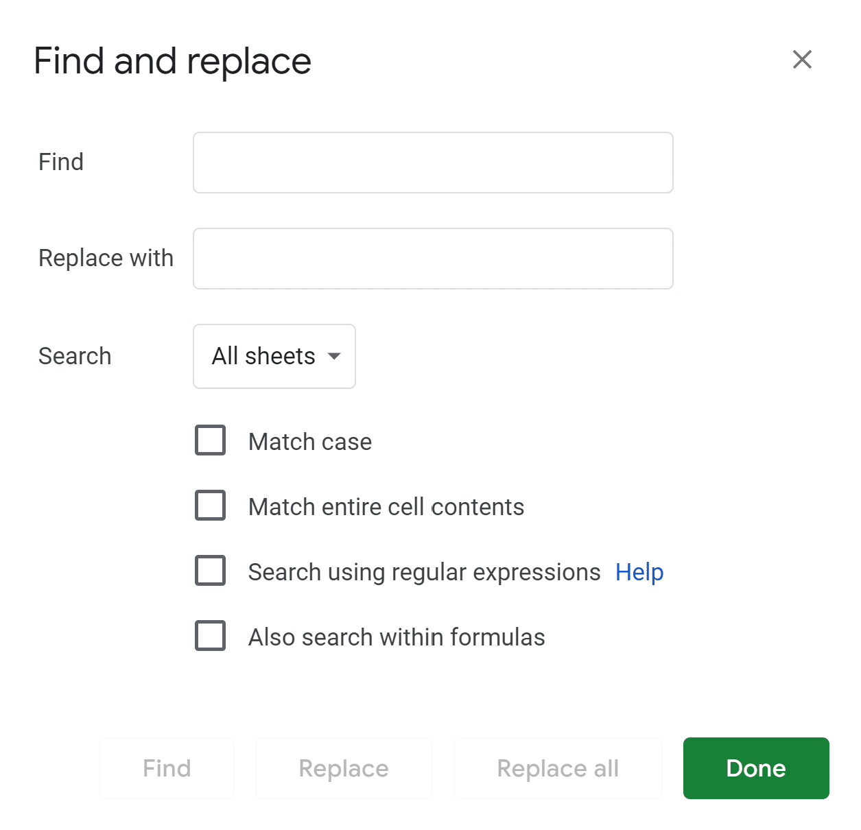
- Navigate to Edit>Find and replace (or press Ctrl+H)
- In the box that pops up, enter the data you want to replace and what you want to replace it with
- Click Done
You can use the dropdown box to only search certain sheets or ranges too.
How to Search in Google Sheets and Highlight the Matching Data
There are different ways you can use this technique:
- Search and Highlight only the cells with the matching data
- Search and Highlight the entire row where there is a match
- Search and Highlight cells/rows even if there is a partial match
In the below section, I will each of these cases in detail and show you how to create this in Google Sheets.
How to Search in a Google Spreadsheet and Highlight Cells with the Matching Data
In this section, I will show you how to create something as shown below:

Note that as soon as I enter the country name in cell B1 and hit Enter, it highlights the matching cells in column B.
Here is how to make this searchable Google spreadsheet:
- Select the data that you want to get highlighted when a match is found. In this example its B4:B12.
- Click on the Format button in the menu.

- Click on Conditional Formatting.

- In the ‘Conditional formatting rules’ pane that open, click on the ‘Format cells if’ option.

- Select the ‘Custom formula is’ option.

- In the Value or Format field, enter the formula: =B4=$B$1

- Specify the formatting style you want to be applied (in this example, I am going with the default green color).
- Click on Done.


Now, whenever you enter any text in cell B1, it will highlight the matching cells in the dataset.
Note that there needs to be an exact match. If the text entered is misspelled, or is partial/incomplete, the cells would not be highlighted.
In the above example, I am entering the data manually. However, if you have a huge dataset, you can create a drop-down list in cell B1. This will allow the user to see all the options in one place and select the required one.
How to Search on a Google Spreadsheet and Highlight Rows where there is a Match
In the above example, we highlighted only the matching cells.
But in a real-world example, you’re more likely to search for a data point and highlight the entire row.
Something like shown below:
Here are the steps you can use to learn how to search on Google Sheets and highlight the entire row in:
- Select the entire data set.
- Click on the Format button in the menu.
- Click on Conditional Formatting.
- In the ‘Conditional formatting rules’ pane that opens, click on the ‘Format cells if’ option.
- Select the ‘Custom formula is’ option.
- In the Value or Format field, enter the formula: =$B4=$B$1
- Specify the formatting style you want to be applied (in this example, I am going with the default green color).
- Click on Done.
How to Search on a Google Sheet and Highlight Rows With Partial Match
In the above examples, it was necessary that there be an exact match for the cells/rows to get highlighted.
But you may have a situation where you want to get match based on the partial search string.
Something as shown below:

Note that here as soon as I entered ‘abc’ in cell A1 (it doesn’t matter whether it’s lower case or upper case), all the rows in the dataset that have that string get highlighted.
Here is how to search in a Google Sheet with the same method as above:
- Select the entire data set.
- Click on the Format button in the menu.
- Click on Conditional Formatting.
- In the ‘Conditional formatting rules’ pane that open, click on the ‘Format cells if’ option.
- Select the ‘Custom formula is’ option.
- In the Value or Format field, enter the formula: =IF($A$1<>””,ISNUMBER(SEARCH($A$1,$A4)),FALSE)
- Specify the formatting style you want to be applied (in this example, I am going with the default green color).
- Click on Done.
In case you want the search to be case sensitive (which means that ‘abc’ and ‘ABC’ are different), then use the FIND function instead of the SEARCH function in the above formula. It’s the best method to use when tackling how to find on Google Sheets.
So this is how to search in Google Sheets and highlight matching data (be it cells or rows)
You may also like the following tutorials:
- Using Query Function in Google Sheets – with Examples.
- How to INDEX MATCH in Google Sheets
- Remove Last Character from a String in Google Sheets
- Conditional Formatting Based on Another Cell Value in Google Sheets
- Ultimate Guide to Conditional Formatting in Google Sheets
- How to Zoom In and Zoom Out in Google Sheets
- Creating a Heat Map in Google Sheets (Step-by-Step Tutorial)
- Creating a Dynamic Filter in Excel (extract data as you type)
- How To Format Phone Numbers In Google Sheets?
- How To Sort by Date in Google Sheets [4 Easy Methods]


3 thoughts on “How to Search in Google Sheets and Highlight Matching Data”
The formula =IF($A$1””,ISNUMBER(SEARCH($A$1,$A4)),FALSE) is not working for me. It says “Invalid Formula”
It took me embarrassingly long: the range of the Conditional Formatting is shown to be A1, but in fact it needs to be the range you wish to highlight: i.e. B4:B (this should get the entire column: the range must start at the cell you identify in the formula, and should auto-update as you add rows)
this does not work for me, and I cannot figure out why
Comments are closed.