Here’s what you need to know about the NPER function in Google Sheets. It’s mainly used to determine the number of payment periods until a debt is paid off. The function assumes a constant interest rate, static payment, and no additional principal additions (aside from interest). Because of that, the Google Sheets NPER function is helpful as a quick payoff calculator in your budget spreadsheet.
So how do you use the NPER function? I’ll walk through the syntax, uses, and other considerations in this guide. Most importantly, I made a free downloadable NPER function template!
This Article Covers:
What is the NPER Function?
NPER is formula-speak for “number of periods”. That makes sense. The NPER function calculates how many payments you’ll need to make to pay off a loan amount, given a static interest rate. There are a couple of important limitations to the NPER function:
- Your interest rate cannot change (be variable) over time.
- You will need to define your interest rates and the payments over the same interval of time (such as annual or monthly).
But if you are able to do these two things, the NPER function is very useful. With the NPER function, you’ll be able to see exactly how many payments you’ll need to make to clear your balance. Just stay on track, and you’ll be done in no time at all.
NPER Function Syntax in Google Sheets
I like to break down formulas by their syntax. It helps me understand what a formula needs if I want to make it work. That applies to NPER in any spreadsheet software (including Excel).
According to Google, the NPER function is built as follows.
=NPER(rate, payment, current value, [future value, when payments are due])
The first three requirements are pretty easy.
- Rate: What’s the current interest rate? Enter this as a percentage.
- Payment: Enter this as a negative value. It’s what you’re paying toward the debt.
- Current Value (or Present Value or PV): How much do you owe right now?
The other two parts are optional. You can enter them if you want to calculate a payoff to a certain amount (aside from 0), and if you want to calculate whether you’re paying at the start or end of the period.
- Future Value (or FV): Do you want to end this calculation at a number other than $0? If so, enter it in this optional argument. That’s the cash balance at the end.
- When Payments are Due (or “End or Beginning”): Are your payments due at the end or the beginning of the month? Enter this as 0 (end/default) or 1 (beginning).
How Do You Use the NPER Function?
Aside from evaluating the syntax, the best way to understand the NPER function is with an example.
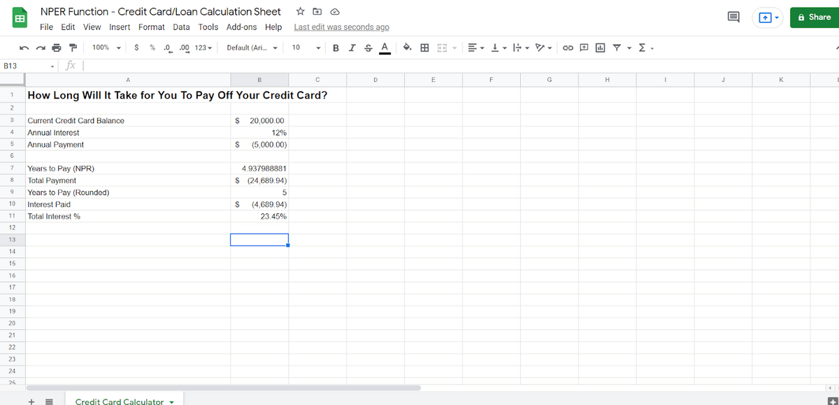
Let’s start building our spreadsheet. Say you currently have a loan with a $20,000 balance (oh no!) and you want to pay $5,000 down on it a year. Those unfamiliar with interest accumulation might think such a debt would only four years to pay off, but that’s not true. With a 12% interest rate, the payments just keep going.
Required Arguments
Let’s start by entering the basics into a spreadsheet. You can do this in Google Sheets or Microsoft Excel.
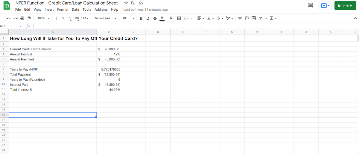
In my screenshot above, I’ve entered all the information we discussed. These are the function’s required arguments. Once we have these, the NPER function calculates the rest.
Here’s what we enter manually:
- Your current card balance.
- Your annual interest rate.
- Your annual payment.
Note that it’s an annual interest rate and an annual payment. Note also that the payment is a negative amount (in parentheses), not a positive amount. And don’t forget about cash flow convention. Incoming money is represented by positive numbers. Since you are paying down the account, you need to have the payment be negative in this cell of the worksheet.
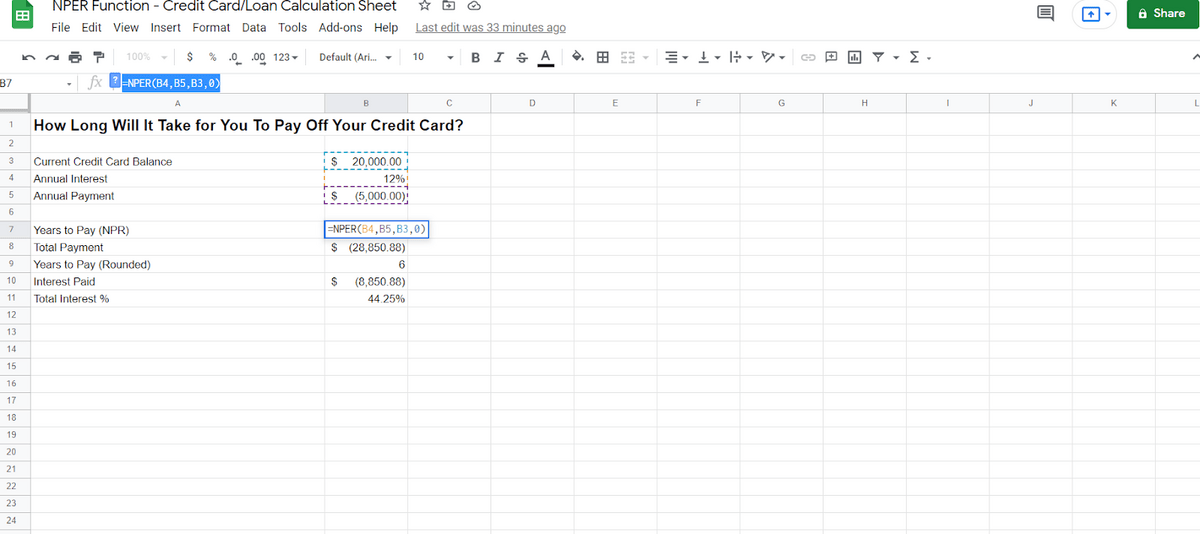
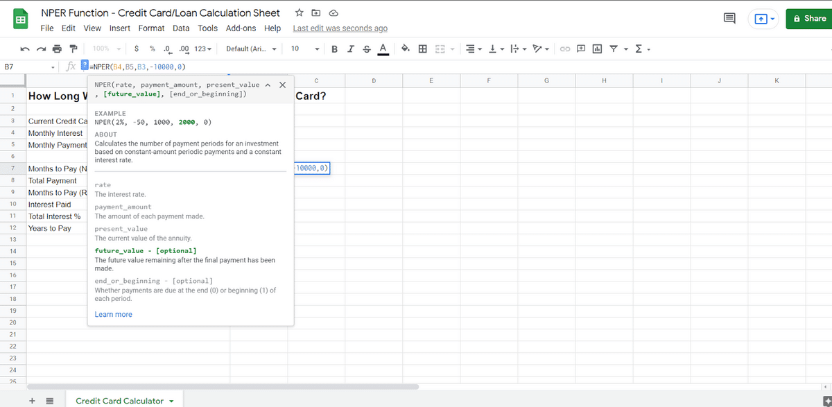
From those manual variables, we’re able to use the Google Sheets NPER function. My screenshot below shows what that looks like. Remember the syntax above. B4 is the interest rate, B5 is the payment, and B3 is the current value (CV).
Look familiar? It should!
Optional Arguments
Now let’s look at those optional arguments I mentioned above.
- Future value: how much you’re hoping to owe.
- End or beginning: when payments are due.
Let’s start with “end or beginning.” By default, the value here is “0.” Let’s turn it to “1” (beginning of the period) and see what happens.
By changing the “end or beginning” argument to “beginning”, it shaved a whole year off my pay-down period! Why?
The lower total payment amount shows how much time (and money) you’d save by paying at the start of the payment period (January 1st, in this case) instead of at the end of it (December 31st of that same year).
Not only does that mean that you have a year less of payments, but it also means that less interest compounds.
Using NPER to Calculate Your Total Payment
As you can see on our sheet, we’ve also calculated total payment. NPER can be used for this purpose; you just multiply the exact NPER by the payments you’re making.
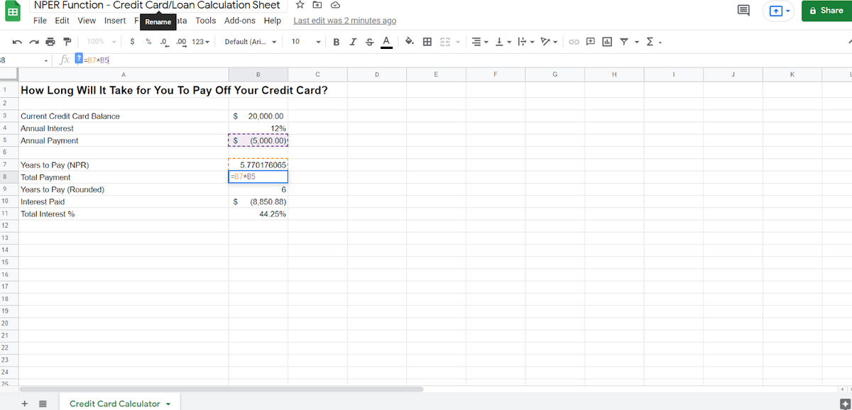
In this case, we can see that over the course of the next six years, we’re going to pay about $8,000 in interest. That’s a lot, but at least it’s spread out. We can also calculate that the total interest paid is about 44.25% of the initially borrowed amount.
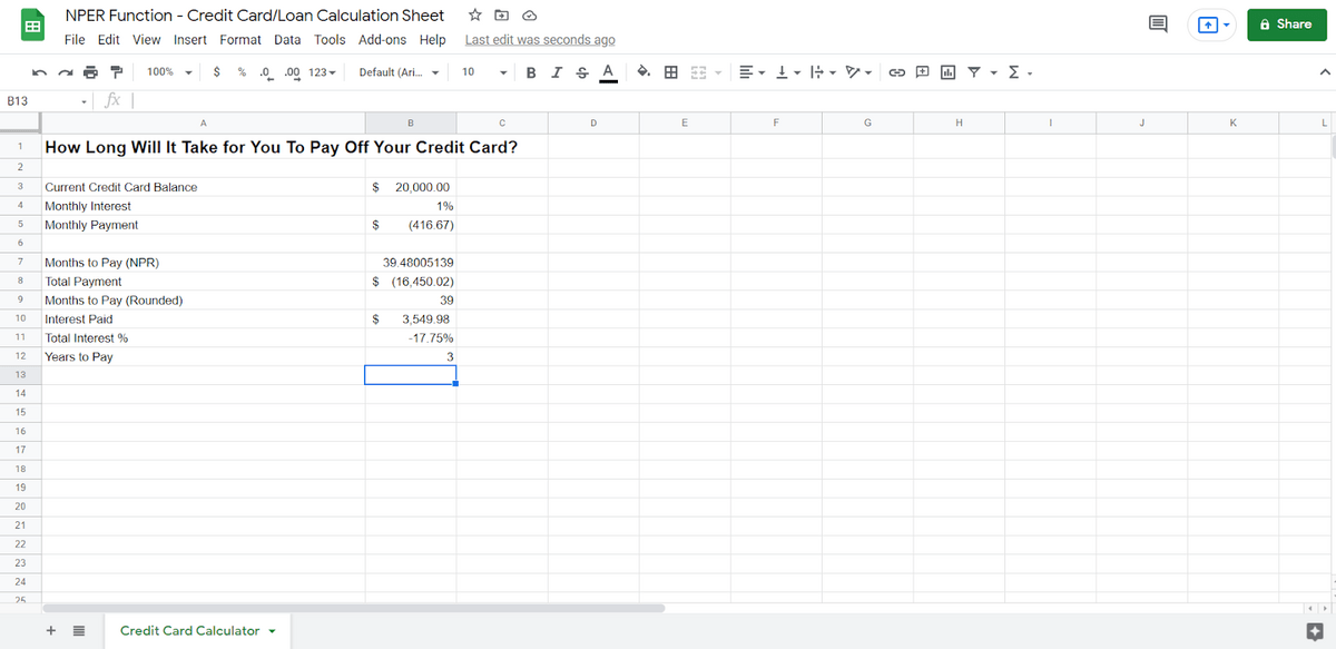
Changing Our NPER to Monthly
Well, obviously a credit card bill is due monthly rather than being due annually. So, maybe we would rather know how much we have to pay every month. All we have to do is change the interval of both the interest rate and also the interval of the payments.
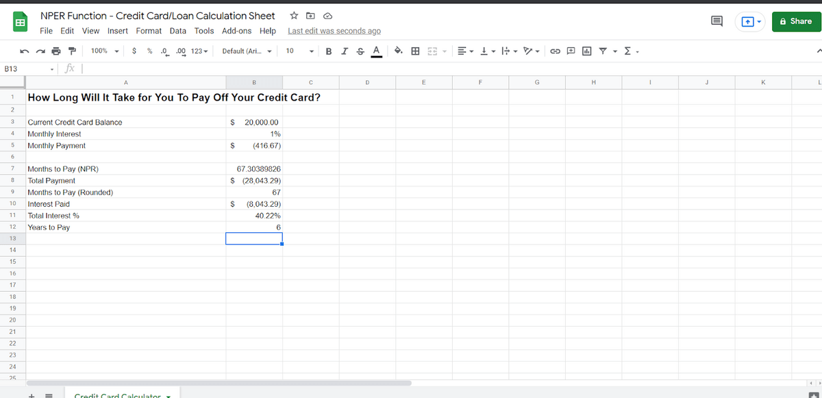
Now, you might notice that the numbers are a little different. There’s a reason for that. Because you’re paying down the balance faster, you’re paying less interest. Our first calculation was annual which meant you had a full year of interest before the first payment. Now, you only have a single month of interest before the first, smaller payment.
It still rounds out to about 6 years to pay, but only just barely — it’s closer to five and a half years. Over the entire time, you’re paying closer to 40% in interest rather than 44.25%.
Calculating a Partial Pay-Off With Google Sheets NPER
Okay, but what if we want to know how long it will take us to pay off half of the balance? We can do that, too. When we first declared NPER, we used “0” as the desired balance, because we wanted to know how long the loan would take to completely pay off. We can modify it like so:
And then we get the following result:
There are a few things to note about this. First, the “future_amount” is a negative number. Otherwise, it won’t calculate properly.
Second, we can see that it’s going to take about 3 years to pay off the loan halfway. (That’s also a case where you may want to check for net present value). And that makes sense. But we also note that we’ve paid about $6,000 in interest already. That’s correct.
Because of compounding interest, you will always be paying more interest and less principle at the beginning of a loan, and less interest and more principle at the end of the loan. Once you reach that halfway point, you’re paying interest on $10,000 rather than the $20,000 at the beginning and this continues to go down.
Can You Use NPER for Something Other Than Loans?
You might have noticed that the amounts you owed were expressed as negatives. You can use NPER to calculate positives as well — such as how much you might want to save for retirement. Take a look at this sheet:
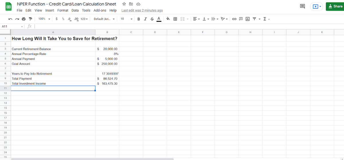
Here, we’ve calculated that it will take 17 years to save $250,000, starting with $20,000 and paying $5,000 each year (and gaining 8% annually). That’s a lot of time, but look at the calculations. You’re only paying $86,000 or so and making a total investment income of around $160,000.
Let’s take a look at the NPER calculations we used.
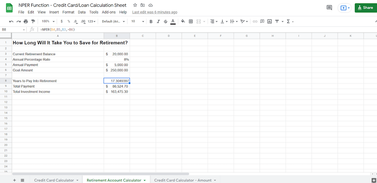
All we had to do was change the signage of the payments and the goals (from negative to positive and vice versa) and we were able to calculate earnings rather than payments.
Calculating How Much to Pay With PMT
All that being said, a lot of people don’t determine how much to pay and then calculate out how many payments there will be. Rather, a lot of people want to know how much they need to pay so they can pay off a balance in a certain amount of time. The payment is a lump-sum amount that pays toward the principal and interest of the loan.
Let’s say you don’t want to spend six years paying off that $20,000 balance. You’d rather pay it off in 4. To do that, you’ll use the related PMT function.
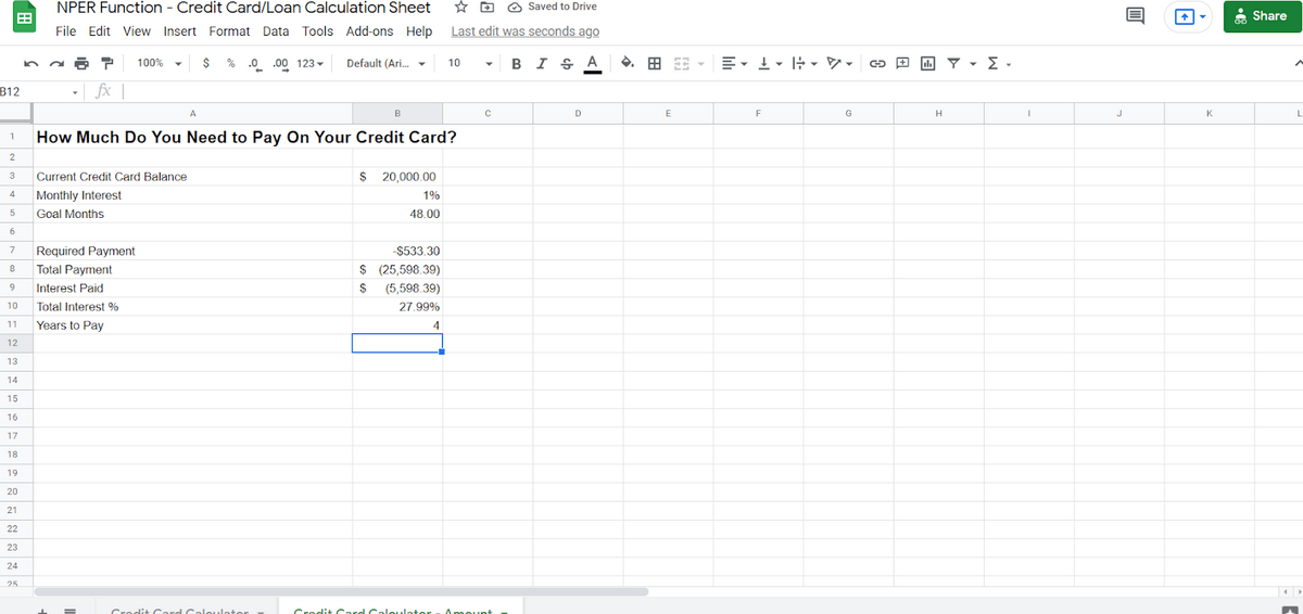
Here, we’ve started with three numbers:
- The current balance.
- The monthly interest.
- The number of months we want to pay the balance off in.
From there, we’ve used the PMT function.
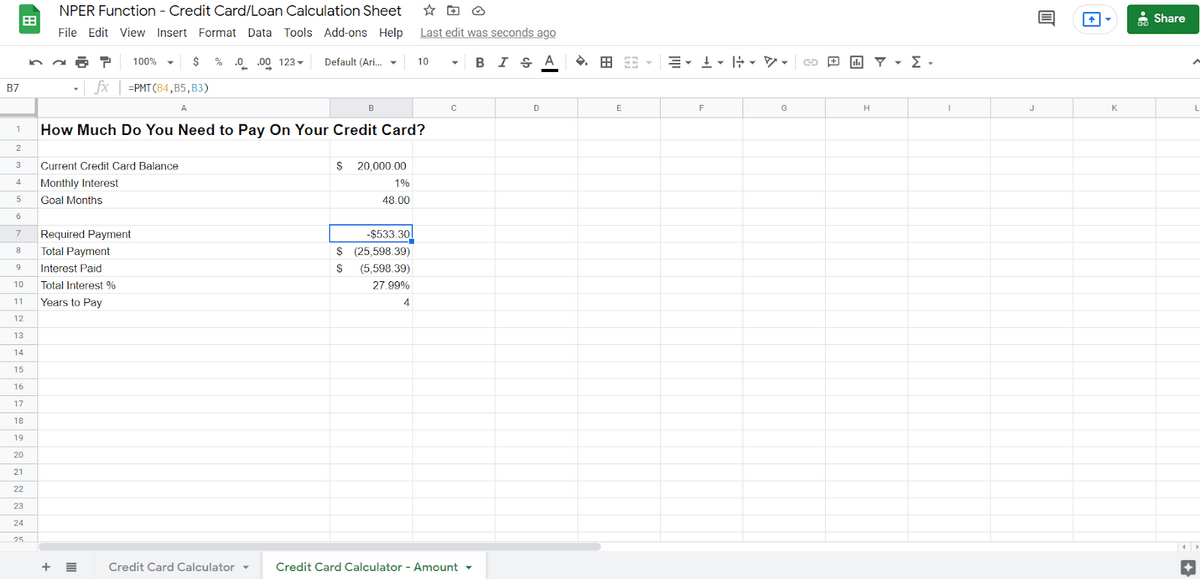
The PMT formula goes like this:
=PMT(rate, number_of_periods, present_value)
In this case, that is 1%, 48, and $20,000. The PMT formula will tell you that you will need to pay $533.30 every month to pay off the balance in 4 years. That’s not a lot more than you were paying in the prior calculations, but it shaves off about 2 years of time and $3,000 in interest.
With NPER and PMT, you can do pretty much anything you need to in terms of calculating your loan payoff amounts and your loan payoff dates.
Google Sheets has quite a few functions that you can use to do extremely complex financial calculations. That’s one reason I took the time to evaluate training courses on the subject. You can use Google Sheets for practically all your financial spreadsheet needs.
Frequently Asked Questions
The NPER formula raises a bunch of questions (especially for those outside the accounting field). Here are some of those I hear most frequently.
What are the limitations of the NPER function?
While it’s super-helpful for evaluating principal and interest payments, it doesn’t take into consideration fees or taxes. It also doesn’t account for payment fluctuations. If you want to make a lump-sum payment, this formula doesn’t take that into consideration.
What is PMT vs PV in a function?
The PMT and PV arguments both appear in the NPER function, but that ask for different things. PMT requests the payment amount (presented as a negative as per cash flow convention). PV requests the present value. I dive further into the syntax of the NPER function above.
Note Excel has a PV function that returns the present value of an investment. You can plug that into the NPER function. Looking for even more ways to connect your data? You can also pull your payment information from another sheet, if needed.
What does NPER mean in Excel?
The NPER function means “number of periods” in both Excel and in Google Sheets. Break NPER apart to see N for Number and PER for Periods. Note that the function works the same way in both spreadsheet tools.
What does NPER do?
NPER calculates the number of periods until you pay off a loan. It’s only used for loans with static payment amounts and constant interest rates. It doesn’t account for taxes, fees, payments in lump-sum amounts. You can use it for any series of future payments in a fixed amount with a fixed interest rate.
Alternately, you can use this to track retirement savings goals where a number of monthly investments never changes and you have a fixed interest rate. It’s a worthwhile consideration if you have a locked rate in a high-yield savings account, for example.
How does the NPER function differ in Excel and Google Sheets?
In either scenario, the NPER function has the same syntax. It always requires interest rate, payment amount, and current value. It also optionally asks for future value and whether to apply payments at the beginning or end of the period.
Why is PMT negative in NPER?
Remember that cash inflows need to be positive when dealing with accounting. Cash outflows are negative. The NPER worksheet function is made for these types of evaluations, so you’ll need to follow this formatting convention.
When would PMT be positive in NPER?
While incoming cash flows are positive, you’d also use a positive PMT amount when using NPER to calculate investment returns.
Why am I seeing a #VALUE! error in NPER formula?
You’ll see a #VALUE! error if you use non-numeric values in the formula. Make sure you’ve formatted your cells correctly, and that you’re pointing the function’s arguments to the right places.
Download My Free NPER Google Sheets Template
If you’re trying to use the NPER function, you can get started with my NPER template. Note that this is the same spreadsheet template I used in my screenshots above. Note that my link allows you to copy the NPER worksheet to your own Google Drive, where you can edit it for your personal or business use.
The NPER function should work to figure out how many payments you need to make to clear your balance — regardless of the type of debt.
Conclusion
For nearly any financial function, Google Sheets will have a correlative function. This also includes tracking investments. In addition to being able to see how much money you need to pay down on a loan, you can also use Google Sheets to see how much you would need to pay toward, for instance, your retirement.
I hope you enjoyed my guide to NPER in Google Sheets. Please let me know if you have any questions in the comments.
Related reading: NPV Google Sheets Formula