Easy Guide to the Google Sheets INDEX Function (4 Examples)

The INDEX function is perhaps one of the most under-used functions in Google Sheets. However, if you know the right way to use it, you’ll find it quite handy in a lot of applications.

In this tutorial, we will show you two ways to use the Google Sheets INDEX function:

• When you want to return a cell value
• When you want it to return an array formula

We will also explain, with the help of examples, how the INDEX function can be applied to extract data from your dataset.

What Does the Google Sheets INDEX Function Do?

The INDEX function in Google Sheets is used to extract data from a cell or range of cells.

We specify which cell or range of cells we want to extract by providing the function with a specific range, a row, and a column.

The INDEX Google Sheet function will return the cell or array of cells at the intersection of the specified row and column of the specified range.  

Syntax of the INDEX Function in Google Sheets

The syntax for the Google spreadsheet INDEX function can be written in two ways:

INDEX(reference, [row], [column])

This is the syntax that uses the cell reference form of input. Here,

• reference is a range of cells from which we want to extract the data.
• row is the row number (within the reference range) from which we want to extract the data.
• column is the column number (within the reference range) from which we want to extract the data. This parameter is optional.

The above syntax will return the value in the cell that is at the intersection of the given row and column index within the range specified in the reference parameter.

For example, take a look at the screenshot below:

If you type the following formula in a cell, it will give you the value at the cell, which is at the intersection of the second row and third column of the range specified in the first parameter:

=INDEX(A2:C3, 2, 3)

The returned value would be 6.

Note: If you set the row or column parameter to 0, the INDEX formula Google Sheets returns an array of values for the entire column or row, respectively.

INDEX(array, row, [column])

This is the syntax that uses the array form of input. Here,

• array is a range of cells or an array constant from which we want to extract the data.
• row is the row in the array from which we want to extract the data. This is optional if the column parameter is specified.
• column is the column in the array from which we want to extract the data. This is optional if the row parameter is specified.

If both row and column parameters are specified, the above syntax will return the value which is at the intersection of the specified row and column.

For example, consider the formula given below:

=INDEX({1, 2; 3, 4}, 1, 2)

In this formula, we provided the Google Sheets INDEX function with a 2×2 array as its first parameter. This array contains 1 and 2 in the first row and 3 and 4 in the second row.

The above formula uses the INDEX function to return the value at row 2 and column 3 of the specified array.

The returned value would be 2.

Note: If you set the row or column parameter to 0, the INDEX function returns an array of values for the entire column or row, respectively.

How to Use the INDEX Function in Google Sheets

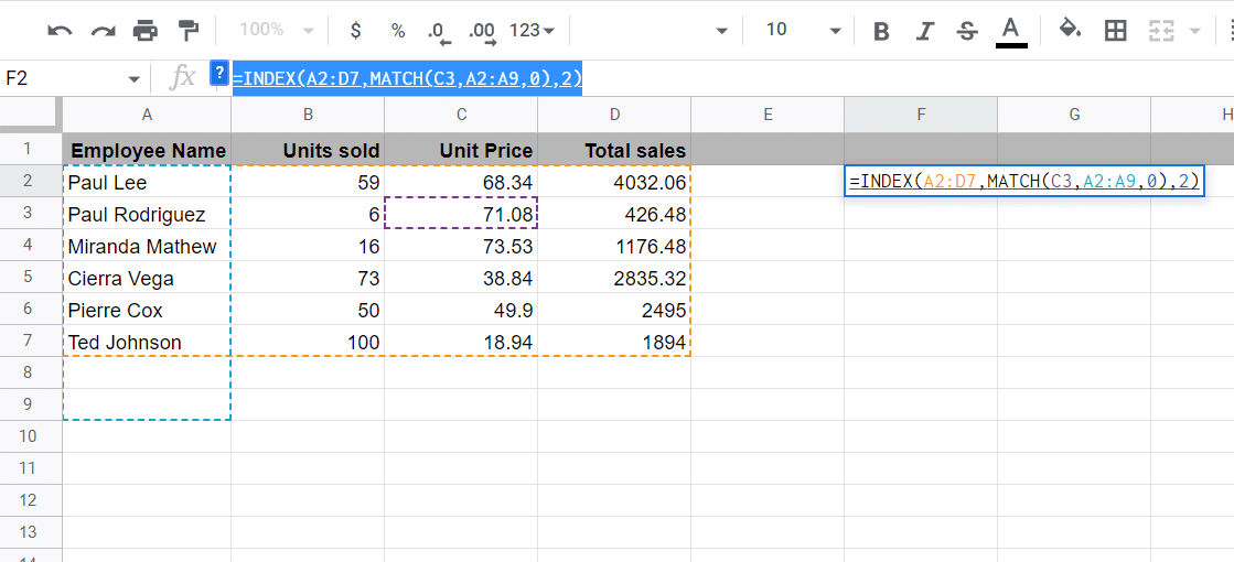
To further understand how to apply the syntaxes shown above, let us use the sample dataset shown below:

The dataset contains employee sales information. Let us use the INDEX function to extract some valuable information from this dataset.

Using the INDEX Function Google Sheets to Return a Cell Value

Let us say you want to know what the total sales that Cierra Vega made were.

You can easily use the INDEX formula to extract this information from the table if you know exactly which row Cierra Vega’s sales information exists.

You also need to know in which column of the selected range, the Total Sales exist.

If we select the range of cells A2:D7, the Total Sales lies in the 4th column, and Cierra Vega’s information lies in the 3rd row of the selection.

So to find out her total sales, we will use the formula:

=INDEX(A2:D7,3,4)

Your results will then be:

In this way, you can use the same formula to extract the contents of any cell in your sheet, simply by changing the references in the INDEX function parameters.

Let us extract a few more values:

Using the INDEX Function to Return an Array Formula

If you want to extract not just the value of one cell, but a whole column or row of cells, then there’s an effective way to use the INDEX Google Sheets function to do this.

Using the INDEX Function to Extract a Row of Data

Let us say you want to know all the information about Cierra Vega. This means you want to extract all four cells from the 3rd row of the table.

For this, you will need the INDEX function to return an array formula that will contain all 4 values of the 3rd row.

So to extract all four cells relating to the 3rd row, we will use the formula:

=ArrayFormula(INDEX (A2:D7,3,0) )

Here are the steps you need to follow:

1. Select the first cell where you want the extracted results to appear.
2. Make sure there are 3 empty cells next to it, so all four extracted values can appear next to each other.
3. In the formula bar, type the formula shown above.
4. Press the return key.
5. You should now be able to see all details relating to Cierra Vega next to each other.

Note that the result that you get is an array and not actual values in the physical cells. So if you make any changes to any of the displayed values, you will get an error.

Explanation of the Formula

The formula works because you passed 3 as the row number and 0 as the column number. Since the third row in the selected range is the row relating to ‘Cierra Vega’’, you get an array containing all the contents of row 3.

Using the INDEX Function to Extract a Column of Data

You can also extract all cell values of a particular column in your range. For example, you can use the following formula to get the names of all the employees:

= ArrayFormula (INDEX(A2:D7,0,1))

Here are the steps you need to follow:

1. Select the first cell of a blank column (where you want the extracted results to appear).
2. In the formula bar, type the formula shown above.
3. Press the return key.
4. You should be able to see a list of all employee names in the new column.

Note that the result that you get is an array and not values in the physical cells. So if you make any changes to any of the displayed values, you will get an error.

Explanation of the Formula

The formula works because you passed 0 as the row number and 1 as the column number. Since the first column in the selected range is the ‘Employee Names’ column, you get an array containing all the contents of column 1.

Above, we showed you two ways of using the Google Sheet INDEX function. In the first method, we showed you how to extract a single cell value from a given range, while in the second method we showed you how to extract a range of cell values from a given range.

Using INDEX With the COUNTA Function

The COUNTA function is used to count cells with any kind of data in them. When used with the INDEX function, they will return the values in the last range whenever the sheet is updated.

For example, if we wanted to find the last value for total sales in our example spreadsheet, we could use the formula:

=INDEX((A2:D7),COUNTA(D2:D7),4)

In this formula, we have A2:D7 which is the entire range of the data.

The COUNTA(D2:D7) counts the number of values in column D in the range.

The number 4 represents the column from which the data will be extracted from.

This is a useful way to find the most recent data in a spreadsheet that is constantly being updated.

Using INDEX With the MATCH Function

The Index and Match functions can also be combined to make a more versatile index match formula. As we have already established, the INDEX function is used to return data from a specified range. On the other hand, the MATCH function returns the position of a value in a range of data.

When used together, the index function uses the MATCH formula as the argument. The match function will show where the value is in the range of data, while the index function will return its corresponding values.

In our sheets above, if we wanted to find the corresponding data for Miranda we would use the The index and match functions together to make the Index match formula:

=INDEX(A2:D7, MATCH(A11, A2:A7,0),2)

Separately, we have the Match formula:

 MATCH(A11, A2:A7,0)

which returns the position for Miranda in the data source.

We used the MATCH formula as the row argument in the index formula

=INDEX(A2:D7, MATCH(A11, A2:A7,0),2) 

Finally, the 2 is a reference for the second column, which has the data for the units sold.

The Google Sheets index match function is useful when you have a large range of data.

INDEX Vs OFFSET in Google Sheets

The offset function in Google Sheets is used to return a reference from a specified range of cells that are a specific number of cells away from a given cell.  

The difference between the index function and the offset are:

• The OFFSET function only requires the starting point to be specified in the formula unlike the INDEX function which requires the entire range to be specified.
• INDEX finds a cell at the intersection of a row and column while the offset returns a reference from a range that is a specific number away from the given cell.
• The syntax for the OFFSET function is OFFSET(cell reference, offset rows, offset columns) with the option of also adding height and width, which shows how much you want to displace the rows and columns.
• The two functions both use dynamic data meaning that they update when the original data is changed.

Frequently Asked Questions

When Should You Not Use INDEX in Google Sheets?

The INDEX function works well instead of the VLOOKUP when you have dynamic data. Since it returns the corresponding value, you shouldn’t use it when you want to find the position of the value in the range. Instead, you should use the MATCH function.

This function is also not volatile, which means that if the data is changed, then the formula won’t update, and you will have to redo it.

Finally, if you are working with data that has been sorted, then you shouldn’t use the INDEX function.

What Are Some Similar Formulae to INDEX in Google Sheets?

The VLOOKUP formula and the MATCH formula in Google Sheets are similar to the INDEX. All these formulas are used in Google Sheets to find data in a dataset and return the corresponding values.

The index and match functions are not that different, except the match function returns the position of a value in a data range. The VLOOKUP formula, unlike the other two, returns values from a static column, so if a new column is added, it returns an error.

Wrapping Up

The Google Sheets index function is a useful tool for returning a specific value from a range. This is the ultimate guide on how to use INDEX in Google Sheets. We hope you found our examples and explanations helpful and easy to understand.

Related:

• What are Wildcards in Google Sheets?
• How to Create a Table of Contents in Google Sheets
• How to VLOOKUP from Another Sheet in Google Sheets
• How to Search in Google Sheets and Highlight Matching Data
• How to VLOOKUP Multiple Columns in Google Sheets