The VLOOKUP Google Sheets Function

The VLOOKUP Google Sheets function can be used to look for a value in a column and when that value is found, return a value from the same row from a specified column.

Now if that description sounds nerdy and difficult, here is another way to understand what this function does.

Suppose you have gone to an expensive restaurant and you are looking at their menu to order something nice (but you also don’t want it to be heavy on the pocket).

So you start scanning the menu and when you find something you like, you move your eyes to the right to see the price of that dish.

That’s exactly how Google Sheet VLOOKUP functions works.

If goes down the column of lists/items, looks for the specified item and then returns its corresponding value from the same row.

But how does VLOOKUP work exactly? If you’re still confused about the Google Sheets VLOOKUP function, just bear with me till we reach the examples section.

But before that, let’s quickly have a look at the syntax of Google Sheets Vlookup Function:

VLOOKUP Syntax Google Sheets

Here’s what the VLOOKUP formula in Google Sheets looks like:

VLOOKUP(search_key, range, index, [is_sorted])

• search_key – This is the value or item you’re looking for. For example, in the case of the restaurant, it would be burger or pizza.
• range – this is the range to be used in the Vlookup function. The left-most column of this range would be searched for the search_key.
• index – this is the column number from where you want to get the result. The first column in the range is 1, the second column is 2, and so on. Note that this value should be between 1 and the total number of columns. If not, then it would return a #VALUE! Error.
• is_sorted – [TRUE by default] – in this argument, you can specify whether you’re looking for an exact match or an approximate match. You can use FALSE for exact match and TRUE for an approximate match. When you use TRUE, the list needs to be sorted in an ascending order. If you don’t specify a value here, it takes TRUE as default.

Now let’s look at some examples to understand how to use Google Sheets Vlookup function in real life scenarios.

VLOOKUP for Dummies: How Does the VLOOKUP Google Sheets Function Work in the Real World?

Example 1: Find Student’s Marks From the List (How to Use VLOOKUP Step by Step)

In the Example below, I have the names of students and their score in a subject (let’s say Math).

As a teacher, you may need to quickly pull the marks of students from a list that could be huge.

Knowing VLOOKUP would be helpful in such cases. Let’s take a look at the steps you’d use to find the score using VLOOKUP.

1. Type =VLOOKUP( into an empty cell
2. Enter the value you’re looking for, it can be a numerical figure, text string, or cell reference. Then enter a comma. In the below example, we used the cell reference E2.
3. Enter the range, and make sure you use absolute references($ before the column and row references). Then add a comma.
4. Enter the index. In the below example we put 2 as we want to return the result from the second column in the specified range. Add another comma.
5. Specify if need to return specific values by entering False or leave it blank to sort in ascending order.

Here is the formula that will give you the marks of the specified students.

=VLOOKUP(E2,$A$2:$B$10,2,False)

Now when you change the name in cell E2, the formula would automatically update and return the marks of that student.

Pro Tip: You can also create a drop down list of students so you don’t have to enter the name manually.

Example 2: Find Student’s Grade using Google Sheets VLOOKUP Function

In Example 1, you looked for an exact match of the name to fetch the marks.

In this example, let me show you how to use the approximate match to get the grades of students based on their marks.

Below is the grade table that would determine the grade of a student:

In this example, we need to find the grades in column C based on the marks (in column B). The grading scale is in E2:F7.

Now before using this, you need to know that the grading range needs to be in the given format. For example, you can not have 0-33, 33-50, 50-70, and so on here. You need to have the numbers that are sorted in an ascending order.

Here is the formula that will give you the grade:

=VLOOKUP(B2,$E$2:$F$7,2)

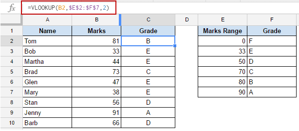
How this works: The VLOOKUP Function looks for the specified score (which is the search_key in this case) and looks for it the ‘Marks Range’ column (which is the left-most column of the lookup range). It goes from top to bottom and when it finds the number which is greater than itself, it returns the grade from the previous row. For example, if the grade is 44, then the function would look through the numbers in E2:E7. Since 0 is less than 44, it moves to 33 which is again lower than 44, so it moves to 50 which is higher. So it goes back to the previous value (which is 33) and returns its grade (which is E).

Example 3: How to Use VLOOKUP in Google Sheets for a Two Way Lookup

What we have seen so far is using Vlookup to return the value from a single column, since we had hard-coded the value. For example, in the case of Example 1, it would always return the score from column 2, as we had hard coded the value 2 in the formula.

However, suppose you have a data set as shown below:

Here, you can use the 2-way lookup technique to fetch the marks for Brad (in cell F4) in Math (in cell G3).

This VLOOKUP Google Sheets example uses the following the formula that will do this:

=VLOOKUP(F4,A2:D10,MATCH(G3,$A$1:$D$1,0),0)

How this works: In this case, to make the subject part dynamic, we have used the MATCH function within the VLOOKUP function. MATCH function looks for the subject name in A1:D1 and returns the column number where it finds the match. This column number is then used in the VLOOKUP function to return the marks of the specified student in that subject.

We hope this VLOOKUP for Dummies article has helped explain how VLOOKUP works in Google Sheets.

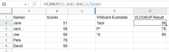
Example 4: How to Use VLOOKUP with a Wildcard for Partial Matches

VLOOKUP can search for partial matches using wildcard operators. The compatible wildcard operators are:

• A question mark ? which can replace a single character
• An asterisk * which can replace a sequence

Note: For the wildcard to work, it needs to be taken from a cell reference and not manually entered into the formula.

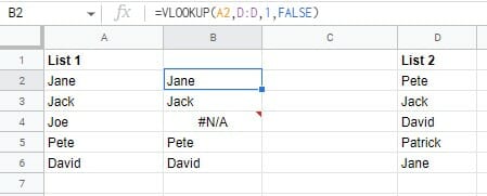
Example 5: How to Do VLOOKUP in Google Sheets When Comparing Data Lists

You can compare two lists by using VLOOKUP.

Let’s say you have two lists of names and need to figure out which is missing from list 1. You could use the following steps to do this:

1. Type =VLOOKUP( into an empty cell
2. Use the first cell from the first list as the search_key (A2 in the below example)
3. Use the second list as the range (we used D:D in the below example to search the entire column)
4. Enter 1 as the index
5. Use FALSE as the is_ascending value
6. Press Enter, then click and drag the formula over the applicable cells in the column

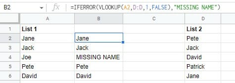
If you want to show something else instead of an #N/A error in the cell you can nest the VLOOKUP function in an IFERROR function like so:

=IFERROR(VLOOKUP(A2,D:D,1,FALSE),"MISSING NAME")

VLOOKUP Function Google Sheets Notes

• VLOOKUP can only look to its right. To search left columns, use MATCH instead.
• VLOOKUP is not case sensitive

Troubleshooting VLOOKUP

Using VLOOKUP in Google Sheets can come with an array of problems, here are a couple of easy fixes that should resolve most of them.

• If is_sorted is omitted or set to true, make sure the first column of range is in ascending order
• If VLOOKUP is returning incorrect results try setting is_sorted to FALSE instead of TRUE or being omitted

How to Do a VLOOKUP in Google Sheets FAQ

What Is VLOOKUP in Google Sheets?

VLOOKUP stands for Vertical Lookup and it allows you to search columns based on the value of another column.

Why use VLOOKUP on Google Sheets Files?

VLOOKUP allows you to perform a range of spreadsheet improving searches, such as:

• Finding incorrect values
• Associating lists
• Checking for missing values between lists that should be identical
• Searching for exact or partial matches to search queries

Why Is My VLOOKUP Not Working In Google Sheets?

Some of the most common errors are:

• Not having a sorted column for the range and then using a TRUE value for the is_ascending part formula
• Trying to search the leftmost columns from a right column, in which case you should use MATCH instead
• Your trying to search with case sensitive queries (VLOOKUP is case insensitive)

Is VLOOKUP Easy to Learn?

VLOOKUP is one of the easier functions to master in Google Sheets. Once you understand the basics you should have no trouble moving forward with your learning.

How Do You Do a VLOOKUP Without Exact Match?

1. Make sure the range column is sorted in ascending order by navigating to Data > Sort sheet
2. Use the formula as you normally would
3. Make sure is_sorted is set to TRUE

You can also use the wildcard operators of * and ? to search partial matches of text strings. For example instead of searching for “James” you could search for “Ja*”

Why Is My VLOOKUP Not Working Until I Click in Cell?

VLOOKUP does not auto-update as it can mess up a lot of other formulas in complex sheets. So, you must manually click the cell to update it.

Related: A detailed guide on using the Excel Vlookup Function.

If You Found This VLOOKUP Google Sheets Tutorial Useful, You May Also Like the Following Articles:

• Get website feed using IMPORTFEED function in Google Sheets.
• Using Query function in Google Sheets.
• Using COUNTIF Function in Google Sheets.
• How to VLOOKUP in Another Sheet in Google Sheets
• How to VLOOKUP Multiple Columns in Google Sheets?
• How to Use the INDEX function in Google Sheets
• How to Use Index Match in Google Sheets (Step-by-Step Guide)